正準判別分析 Last modified: Jul 06, 2015
目的
正準判別分析を行う。
MASS パッケージにある lda は,3群以上の判別の場合には,正準判別分析を行っている。
そして,このプログラムも lda も,全く同じ答えを出す。
使用法
candis(data, group)
print.candis(obj)
summary.candis(obj)
plot.candis(obj, pch=as.integer(obj$group), col=as.integer(obj$group))
引数
data データ行列(行がケース,列が変数)
group 各ケースがどの群であるかを表す変数
obj candis が返すオブジェクト
3 群以上の判別図
pch プロット記号(判別する群の数と同じ長さの整数ベクトル)
col プロット色(判別する群の数と同じ長さの整数ベクトル)
xpos, ypos legend 関数の x, y 引数(座標値の他,xpos="topright" など)
... plot への引数
2 群の判別図
which 図の種類 boxplot か barplot
nclass barplot のときのおよその階級数
... boxplot, barplot への引数
ソース
以下のほかに,一般化固有値問題を解く関数が必要。
インストールは,以下の 1 行をコピーし,R コンソールにペーストする
source("http://aoki2.si.gunma-u.ac.jp/R/src/candis.R", encoding="euc-jp")
# 正準判別分析
candis <- function( data, # 説明変数データ行列
group) # 群変数
{
vnames <- colnames(data)
group <- as.factor(as.matrix(group)) # 群を factor に変換
OK <- complete.cases(data, group) # 欠損値を持つケースを除く
data <- as.matrix(data[OK,])
colnames(data) <- vnames
group <- group[OK]
p <- ncol(data) # 変数の個数
n <- nrow(data) # ケース数
n.i <- table(group) # 各群のケース数
k <- length(n.i) # 群の個数
group.means <- matrix(unlist(by(data, group, colMeans)), p) # 各変数の群ごとの平均値
grand.means <- colMeans(data) # 各変数の全体の平均値
means <- cbind(grand.means, group.means) # 結果表示のためにまとめる
F.value <- apply(data, 2, function(x) oneway.test(x ~ group, var.equal=TRUE)$statistic)
df1 <- k-1
df2 <- n-k
p.value <- format.pval(pf(F.value, df1, df2, lower.tail=FALSE))
wilksFromF <- df2/(F.value*df1+df2)
univariate <- data.frame(wilksFromF, F.value, rep(df1, p), rep(df2, p), p.value)
ss <- split(data.frame(data), group)
w <- Reduce("+", lapply(ss, function(x) var(x)*(nrow(x)-1))) # 群内変動・共変動行列
b <- (var(data)*(n-1))-w # 群間変動・共変動行列
within.cov <- w/(n-k) # プールされた分散・共分散行列
sd <- sqrt(diag(within.cov))
within.r <- within.cov/outer(sd, sd)
result <- geneig(b, w) # 一般化固有値問題を解く
eigen.values <- result$values # 固有値
nax <- sum(eigen.values > 1e-10) # 解の個数
eigen.values <- eigen.values[1:nax] # 必要な個数の固有値を取り出す
eigen.vectors <- result$vectors[, 1:nax,drop=FALSE] # 固有ベクトルも取り出す
LAMBDA <- rev(cumprod(1/(1+rev(eigen.values)))) # Wilks のΛ
chi.sq <- ((p+k)/2-n+1)*log(LAMBDA) # カイ二乗値
l.L <- 1:nax-1
df <- (p-l.L)*(k-l.L-1) # 自由度
p.wilks <- pchisq(chi.sq, df, lower.tail=FALSE) # P 値
canonical.corr.coef <- sqrt(eigen.values/(1+eigen.values)) # 正準相関係数
temp <- diag(t(eigen.vectors) %*% w %*% eigen.vectors)
temp <- 1/sqrt(temp/(n-k))
coeff <- eigen.vectors*temp # 正準判別係数
const <- as.vector(-grand.means %*% coeff) # 定数項
coefficient <- rbind(coeff,const) # 両方併せる
std.coefficient <- coeff * sqrt(diag(within.cov)) # 標準化正準判別係数
centroids <- t(t(coeff) %*% group.means+const) # 重心
can.score <- t(t(data %*% coeff)+const) # 正準得点
structure <- matrix(0, p, nax) # 構造行列
for (i in 1:nax) {
ss <- split(data.frame(cs=can.score[,i], data), group)
ss <- Reduce("+", lapply(ss, function(x) var(x)*(nrow(x)-1)))
structure[,i] <- (ss[,1] / sqrt(ss[1,1] * diag(ss)))[-1]
}
d <- sapply(1:k, function(i) colSums((t(can.score)-centroids[i,])^2)) # 二乗距離
p <- pchisq(d, p, lower.tail=FALSE) # ケースがそれぞれの群に属するとしたとき,その判別値を取る確率
p.Bayes <- t(t(exp(-d/2))*as.numeric(n.i)) # 各ケースが各群に所属するベイズ確率
p.Bayes <- p.Bayes/rowSums(p.Bayes) # P 値
gname <- levels(group)
classification <- factor(gname[max.col(p.Bayes)], levels=gname)
colnames(means) <- c("grand mean", gname)
colnames(univariate) <- c("Wilks のラムダ", "F 値", "df1", "df2", "P 値")
rownames(std.coefficient) <- rownames(structure) <- rownames(univariate) <- rownames(means)
colnames(std.coefficient) <- colnames(structure) <- colnames(coefficient) <-
colnames(centroids) <- colnames(can.score) <- paste("axis", 1:nax)
rownames(coefficient) <- c(rownames(means), "constant")
rownames(centroids) <- colnames(p.Bayes) <- colnames(p) <- gname
rownames(can.score) <- rownames(p.Bayes) <- rownames(p) <- paste("case", 1:n)
return(structure(list(means=means, univariate=univariate, betwee.ss=b, within.ss=w, within.cov=within.cov,
within.r=within.r, eigen.values=eigen.values, LAMBDA=LAMBDA,
chi.sq=chi.sq, df=df, p.wilks=p.wilks,
canonical.corr.coef=canonical.corr.coef, std.coefficient=std.coefficient,
structure=structure, coeff=coefficient, centroids=centroids, can.score=can.score,
p.Bayes=p.Bayes, p=p, classification=classification, group=group, ngroup=k, nax=nax),
class="candis"))
}
# print メソッド
print.candis <- function( obj, # candis が返すオブジェクト
digits=5) # 結果の表示桁数
{
cat("\nWilks のラムダ\n\n")
d <- data.frame(1:obj$nax, obj$LAMBDA, obj$chi.sq, obj$df, format.pval(obj$p.wilks))
colnames(d) <- c("関数", "Wilks のラムダ", "カイ二乗値", "自由度", "P 値")
print(d, digits=digits, row.names=FALSE)
cat("\n判別係数\n\n")
print(round(obj$coeff, digits=digits))
cat("\n標準化判別係数\n\n")
print(round(obj$std.coefficient, digits=digits))
cat("\n構造行列\n\n")
print(round(obj$structure, digits=digits))
cat("\n判別結果\n\n")
print(xtabs(~obj$group+obj$classification))
}
# summary メソッド
summary.candis <- function( obj, # candis が返すオブジェクト
digits=5) # 結果の表示桁数
{
print.default(obj, digits=digits)
}
# plot メソッド
plot.candis <- function(obj, # candis が返すオブジェクト
pch=1:obj$ngroup, # 3 群以上の判別時の記号
col=1:obj$ngroup, # 3 群以上の判別時の色
xpos="topright", ypos=NULL, # 3 群以上の判別時の legend 関数の x, y 引数
which=c("boxplot", "barplot"), # 2 群判別のときのグラフの種類
nclass=20, # barplot のおよその階級数
...) # plot, boxplot, barplot への引数
{
score <- obj$can.score
group <- obj$group
if (ncol(score) >= 2) {
int.group <- as.integer(group)
plot(score, pch=pch[int.group], col=col[int.group], ...)
legend(x=xpos, y=ypos, legend=levels(group), pch=pch, col=col)
}
else {
which <- match.arg(which)
if (which == "boxplot") { # boxplot
plot(score ~ group, xlab="群", ylab="判別値", ...)
}
else { # barplot
tbl <- table(group, cut(score, breaks=pretty(score, n=nclass)))
barplot(tbl, beside=TRUE, legend=TRUE, ...)
}
}
}
使用例
> data(iris)
> (result <- candis(iris[1:4], iris[5]))
print メソッドでは以下の結果だけを表示する
Wilks のラムダ
関数 Wilks のラムダ カイ二乗値 自由度 P 値
1 0.023439 546.12 8 < 2.22e-16
2 0.777973 36.53 3 5.7861e-08
判別係数
axis 1 axis 2
Sepal.Length 0.82938 0.02410
Sepal.Width 1.53447 2.16452
Petal.Length -2.20121 -0.93192
Petal.Width -2.81046 2.83919
constant 2.10511 -6.66147
標準化判別係数
axis 1 axis 2
Sepal.Length 0.42695 0.01241
Sepal.Width 0.52124 0.73526
Petal.Length -0.94726 -0.40104
Petal.Width -0.57516 0.58104
構造行列
axis 1 axis 2
Sepal.Length -0.22260 0.31081
Sepal.Width 0.11901 0.86368
Petal.Length -0.70607 0.16770
Petal.Width -0.63318 0.73724
判別結果
obj$classification
obj$group setosa versicolor virginica
setosa 50 0 0
versicolor 0 48 2
virginica 0 1 49
> summary(result)
sumamry メソッドでは,すべての要素を表示することができる。
$means # 全体および各群の平均値
grand mean setosa versicolor virginica
Sepal.Length 5.8433 5.006 5.936 6.588
Sepal.Width 3.0573 3.428 2.770 2.974
Petal.Length 3.7580 1.462 4.260 5.552
Petal.Width 1.1993 0.246 1.326 2.026
$univariate # 平均値の差の検定(一変量;一元配置分散分析)
Wilks のラムダ F 値 df1 df2 P 値
Sepal.Length 0.38129427 119.26450 2 147 < 2.22e-16
Sepal.Width 0.59921715 49.16004 2 147 < 2.22e-16
Petal.Length 0.05862828 1180.16118 2 147 < 2.22e-16
Petal.Width 0.07111707 960.00715 2 147 < 2.22e-16
$between.ss # 群間平方和・積和行列
Sepal.Length Sepal.Width Petal.Length Petal.Width
Sepal.Length 63.212 -19.953 165.25 71.279
Sepal.Width -19.953 11.345 -57.24 -22.933
Petal.Length 165.248 -57.240 437.10 186.774
Petal.Width 71.279 -22.933 186.77 80.413
$within.ss # 群内平方和・積和行列
Sepal.Length Sepal.Width Petal.Length Petal.Width
Sepal.Length 38.956 13.6300 24.6246 5.6450
Sepal.Width 13.630 16.9620 8.1208 4.8084
Petal.Length 24.625 8.1208 27.2226 6.2718
Petal.Width 5.645 4.8084 6.2718 6.1566
$within.cov # プールした分散・共分散行列
Sepal.Length Sepal.Width Petal.Length Petal.Width
Sepal.Length 0.265008 0.092721 0.167514 0.038401
Sepal.Width 0.092721 0.115388 0.055244 0.032710
Petal.Length 0.167514 0.055244 0.185188 0.042665
Petal.Width 0.038401 0.032710 0.042665 0.041882
$within.r # プールした相関係数行列
Sepal.Length Sepal.Width Petal.Length Petal.Width
Sepal.Length 1.00000 0.53024 0.75616 0.36451
Sepal.Width 0.53024 1.00000 0.37792 0.47053
Petal.Length 0.75616 0.37792 1.00000 0.48446
Petal.Width 0.36451 0.47053 0.48446 1.00000
$eigen.values # 固有値
[1] 32.19193 0.28539
$LAMBDA # Wilks のラムダ
[1] 0.023439 0.777973
$chi.sq # カイ二乗値(近似値)
[1] 546.12 36.53
$df # 自由度
[1] 8 3
$p.wilks # P 値
[1] 8.8708e-113 5.7861e-08
$canonical.corr.coef # 正準相関係数
[1] 0.98482 0.47120
$std.coefficient # 標準化判別係数
axis 1 axis 2
Sepal.Length 0.42695 0.012408
Sepal.Width 0.52124 0.735261
Petal.Length -0.94726 -0.401038
Petal.Width -0.57516 0.581040
$structure # 構造行列
axis 1 axis 2
Sepal.Length -0.22260 0.31081
Sepal.Width 0.11901 0.86368
Petal.Length -0.70607 0.16770
Petal.Width -0.63318 0.73724
$coeff # 判別係数(生データに対応するもの)
axis 1 axis 2
Sepal.Length 0.82938 0.024102
Sepal.Width 1.53447 2.164521
Petal.Length -2.20121 -0.931921
Petal.Width -2.81046 2.839188
constant 2.10511 -6.661473
$centroids # 各群の重心
axis 1 axis 2
setosa 7.6076 0.21513
versicolor -1.8250 -0.72790
virginica -5.7826 0.51277
$can.score # 各ケースの判別スコア
axis 1 axis 2
case 1 8.06180 0.3004206
case 2 7.12869 -0.7866604
case 3 7.48983 -0.2653845
case 4 6.81320 -0.6706311
case 5 8.13231 0.5144625
【中略】
case 147 -5.17956 -0.3634750
case 148 -4.96774 0.8211405
case 149 -5.88615 2.3450905
case 150 -4.68315 0.3320338
$p.Bayes # 各ケースが各群に所属するベイズ確率
setosa versicolor virginica
case 1 1.0000e+00 3.8964e-22 2.6112e-42
case 2 1.0000e+00 7.2180e-18 5.0421e-37
case 3 1.0000e+00 1.4638e-19 4.6759e-39
case 4 1.0000e+00 1.2685e-16 3.5666e-35
case 5 1.0000e+00 1.6374e-22 1.0826e-42
【中略】
case 147 4.6166e-36 5.8988e-03 9.9410e-01
case 148 5.5490e-35 3.1459e-03 9.9685e-01
case 149 1.6137e-40 1.2575e-05 9.9999e-01
case 150 2.8580e-33 1.7542e-02 9.8246e-01
$p # ケースがそれぞれの群に属するとしたとき,その判別値をとる確率
setosa versicolor virginica
case 1 9.9469e-01 1.7650e-20 2.2729e-40
case 2 8.7264e-01 1.6010e-16 2.3190e-35
case 3 9.9309e-01 5.7625e-18 3.6980e-37
case 4 8.4147e-01 2.3946e-15 1.4239e-33
case 5 9.8525e-01 7.0052e-21 8.8231e-41
【中略】
case 147 2.1872e-34 2.2556e-02 8.8926e-01
case 148 3.0565e-33 1.5412e-02 9.4386e-01
case 149 2.8248e-39 3.2602e-05 4.9821e-01
case 150 1.1969e-31 5.4196e-02 8.7125e-01
$classification # 分類された群
[1] setosa setosa setosa setosa setosa setosa setosa setosa setosa
[10] setosa setosa setosa setosa setosa setosa setosa setosa setosa
[19] setosa setosa setosa setosa setosa setosa setosa setosa setosa
【中略】
[136] virginica virginica virginica virginica virginica virginica virginica virginica virginica
[145] virginica virginica virginica virginica virginica virginica
Levels: setosa versicolor virginica
$group # 実際の群
[1] setosa setosa setosa setosa setosa setosa setosa setosa setosa
[10] setosa setosa setosa setosa setosa setosa setosa setosa setosa
[19] setosa setosa setosa setosa setosa setosa setosa setosa setosa
【中略】
[136] virginica virginica virginica virginica virginica virginica virginica virginica virginica
[145] virginica virginica virginica virginica virginica virginica
Levels: setosa versicolor virginica
$ngroup # 群の数
[1] 3
$nax # 解の数
[1] 2
> plot(result, xpos="top")
plot メソッドにより,判別図を描くことができる
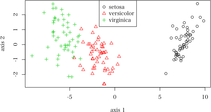 (主成分分析の結果と比較してみよ)
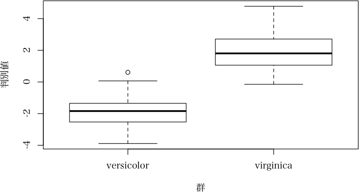
二群判別の場合
> ( result2 <- candis(iris[51:150, 1:4], iris[51:150, 5]) )
判別係数
axis 1
Sepal.Length 0.94312
Sepal.Width 1.47943
Petal.Length -1.84845
Petal.Width -3.28473
constant 4.41899
判別結果
classification
group versicolor virginica
versicolor 48 2
virginica 1 49
> plot(result2)
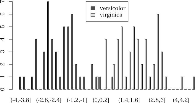
 > plot(result2, which="barplot", nclass=40, args.legend=list(x="top"))
 解説ページ
解説ページ
直前のページへ戻る E-mail to Shigenobu AOKI
