判別分析(ステップワイズ変数選択) Last modified: Aug 25, 2009
目的
ステップワイズ変数選択による判別分析を行う
使用法
sdis(data, group, stepwise=TRUE, P.in=0.05, P.out=0.05, predict=FALSE, verbose=TRUE)
引数
data 説明変数だけのデータフレーム
group 群を表す変数(ベクトルではなく,1 列のデータフレームとして引用するほうがよい)
stepwise ステップワイズ変数選択をするかどうか(デフォールトは TRUE)
P.in Pin(デフォルトは 0.05)
P.out Pout(デフォルトは 0.05,Pout ≧ Pin のこと)
predict 個々の判別結果などを出力するかどうか(デフォルトは FALSE)
verbose ステップワイズ変数選択の途中結果を出力する
分類関数など,予測値など,予測結果集計表に関する結果はそれぞれ,「分類関数」,「個々の判別」,「判別結果集計表」の要素名で参照できる。
2群判別の場合のみ,plot メソッドとして,2 種類の結果グラフ表示を用意している(このページの下の方を参照)。
ソース
インストールは,以下の 1 行をコピーし,R コンソールにペーストする
source("http://aoki2.si.gunma-u.ac.jp/R/src/sdis.R", encoding="euc-jp")
sdis <- function( data, # 説明変数だけのデータフレーム
group, # 群を表す変数(ベクトルではなく,1 列のデータフレームとして引用するほうがよい)
stepwise=TRUE, # ステップワイズ変数選択をする
P.in=0.05, # Pin
P.out=0.05, # Pout (Pout ≧ Pin のこと)
predict=FALSE, # 各ケースの予測値を出力する
verbose=TRUE) # ステップワイズ変数選択の途中結果を出力する
{
step.out <- function(isw) # 変数選択の途中結果を出力
{
step <<- step+1 # ステップ数
ncase.k <- ncase-ng
if (isw != 0 && verbose) {
cat(sprintf("\n***** ステップ %i ***** ", step))
cat(sprintf("%s変数: %s\n", c("編入", "除去")[isw], vname[ip]))
}
lxi <- lx[1:ni]
lxi2 <- cbind(lxi, lxi)
a <- matrix(0, ni, ng)
a0 <- numeric(ng)
for (g in 1:ng) {
a[, g] <- -(w[lxi, lxi]%*%Mean[lxi, g])*2*ncase.k
a0[g] <- Mean[lxi, g]%*%w[lxi, lxi]%*%Mean[lxi, g]*ncase.k
}
idf1 <- ng-1
idf2 <- ncase-(ng-1)-ni
temp <- idf2/idf1
f <- t[lxi2]/w[lxi2] # 偏 F 値
f <- temp*(1-f)/f
P <- pf(f, idf1, idf2, lower.tail=FALSE) # P 値
rownames(a) <- c(vname[lxi])
result2 <- data.frame(rbind(a, a0), f=c(f, NA), p=c(format.pval(P, 3, 1e-3), NA))
dimnames(result2) <- list(c(vname[lxi], "定数項"), c(grp.lab, "偏F値", "P値"))
class(result2) <- c("sdis", "data.frame") # print.sdis を使うための設定
if (verbose) {
cat("\n***** 分類関数 *****\n")
print(result2)
}
alp <- ng-1
b <- ncase-1-0.5*(ni+ng)
qa <- ni^2+alp^2
c <- 1
if (qa != 5) {
c <- sqrt((ni^2*alp^2-4)/(qa-5))
}
df1 <- ni*alp # 第1自由度
df2 <- b*c+1-0.5*ni*alp # 第2自由度
wl <- detw/dett # ウィルクスの Λ
cl <- exp(log(wl)/c)
f <- df2*(1-cl)/(df1*cl) # 等価な F 値
p <- pf(f, df1, df2, lower.tail=FALSE) # P 値
if (verbose) {
cat(sprintf("ウィルクスのΛ: %.5g\n", wl))
cat(sprintf("等価なF値: %.5g\n", f))
cat(sprintf("自由度: (%i, %.2f)\n", df1, df2))
cat(sprintf("P値: %s\n", format.pval(p, 3, 1e-3)))
}
return(result2)
}
fmax <- function() # モデルに取り入れる変数の探索
{
kouho <- 1:p
if (ni > 0) {
kouho <- (1:p)[-lx[1:ni]]
}
kouho <- cbind(kouho, kouho)
temp <- w[kouho]/t[kouho]
temp <- (1-temp)/temp
ip <- which.max(temp)
return(c(temp[ip], kouho[ip]))
}
fmin <- function() # モデルから捨てる変数の探索
{
kouho <- cbind(lx[1:ni], lx[1:ni])
temp <- t[kouho]/w[kouho]
temp <- (1-temp)/temp
ip <- which.min(temp)
return(c(temp[ip], lx[ip]))
}
sweep.sdis <- function(r, det) # 掃き出し法
{
ap <- r[ip, ip]
if (abs(ap) <= EPSINV) {
stop("正規方程式の係数行列が特異行列です")
}
det <- det*ap
for (i in 1:p) {
if (i != ip) {
temp <- r[ip, i]/ap
for (j in 1:p) {
if (j != ip) {
r[j, i] <- r[j, i]-r[j, ip]*temp
}
}
}
}
r[,ip] <- r[,ip]/ap
r[ip,] <- -r[ip,]/ap
r[ip, ip] <- 1/ap
return(list(r=r, det=det))
}
discriminant.function <- function() # 判別係数を計算する
{
lxi <- lx[1:ni]
ncase.k <- ncase-ng
cat("\n***** 判別関数 *****\n")
for (g1 in 1:(ng-1)) {
for (g2 in (g1+1):ng) {
xx <- Mean[lxi, g1]-Mean[lxi, g2]
fn <- w[lxi, lxi]%*%xx*ncase.k
fn0 <- -sum(fn*(Mean[lxi, g1]+Mean[lxi, g2])*0.5)
dist <- sqrt(sum(xx*fn))
errorp <- pnorm(dist*0.5, lower.tail=FALSE)
result3 <- data.frame(判別係数= c(fn, fn0), 標準化判別係数=c(sd[lxi]*fn, NA))
rownames(result3) <- c(vname[lxi], "定数項")
class(result3) <- c("sdis", "data.frame") # print.sdis を使うための設定
cat(sprintf("\n%s と %s の判別\n", grp.lab[g1], grp.lab[g2]))
cat(sprintf("マハラノビスの汎距離: %.5f\n", dist))
cat(sprintf("理論的誤判別率: %s\n", format.pval(errorp, 3, 1e-3)))
print(result3)
}
}
return(list(fn=fn, fn0=fn0))
}
proc.predict <- function(ans)
{
nc0 <- 0
ncase.k <- ncase-ng
lxi <- lx[1:ni]
data <- as.matrix(data)[, lxi, drop=FALSE] # モデル中の独立変数を順序通りに取り出す
dis <- matrix(0, ncase, ng)
for (g in 1:ng) { # 各群の中心までの距離を計算する
xx <- t(t(data)-Mean[lxi, g])
dis[,g] <- rowSums(xx%*%w[lxi, lxi]*xx*ncase.k)
}
pred.group <- grp.lab[apply(dis, 1, which.min)] # 判別された群
P <- pchisq(dis, p, lower.tail=FALSE) # その群に属するとしたとき,距離がそれより大きくなる確率
result4 <- data.frame(実際の群=group, 判別された群 =pred.group,
正否 =ifelse(group==pred.group, " ", "##"), dis,
matrix(format.pval(P, 3, 1e-3), ncase))
colnames(result4)[4:(3+2*ng)] <- c(paste("二乗距離", 1:ng, sep=""), paste("P値", 1:ng, sep=""))
if (ng == 2) { # 判別値を計算するのは2群判別の場合のみ
fn <- ans$fn # 判別係数
fn0 <- ans$fn0 # 定数項
result4$dfv <- data%*%fn+fn0 # 判別値
colnames(result4)[8] <- "判別値"
}
class(result4) <- c("sdis", "data.frame") # print.sdis を使うための設定
result5 <- xtabs(~result4$実際の群+result4$判別された群) # 判別結果集計表
temp <- dimnames(result5)
dimnames(result5) <- list(実際の群=temp[[1]], 判別された群=temp[[2]])
return(list(result4=result4, result5=result5))
}
############## 関数本体
EPSINV <- 1e-6 # 特異行列の判定値
if (P.out < P.in) { # Pout ≧ Pin でなければならない
P.out <- P.in
}
step <- 0 # step.out にて,大域代入される
p <- ncol(data) # 説明変数の個数
if (p == 1) {
stepwise <- FALSE
}
vname <- colnames(data) # 変数名(なければ作る)
if (is.null(vname)) {
vname <- colnames(data) <- paste("x", 1:p, sep="")
}
gname <- names(group)
group <- factor(as.matrix(group)) # 群を表す変数を取り出す(factor にしておく)
ok <- complete.cases(data, group) # 欠損値を含まないケース
data <- as.data.frame(data[ok,])
group <- group[ok]
ncase <- nrow(data) # ケース数
grp.lab <- levels(group) # 群の名前
ng <- nlevels(group) # 群の個数
if (ng <= 1) {
stop("1群しかありません")
}
split.data <- split(data, group)
Mean <- cbind(matrix(sapply(split.data, colMeans), ncol=ng), colMeans(data))
dimnames(Mean) <- list(vname, c(grp.lab, "全体"))
num <- c(sapply(split.data, nrow), ncase)
if (verbose) {
cat(sprintf("有効ケース数: %i\n", ncase))
cat(sprintf("群を表す変数: %s\n\n", gname))
cat("***** 平均値 *****\n")
print(Mean)
}
if (any(num < 2)) {
stop("ケース数が1以下の群があります")
}
t <- var(data)*(ncase-1)
w <- matrix(colSums(t(matrix(sapply(split.data, var), ncol=ng))*(num[1:ng]-1)), p)
dimnames(w) <- dimnames(t)
detw <- dett <- 1
sd2 <- sqrt(diag(w)/ncase)
r <- w/outer(sd2, sd2)/ncase
if (verbose) {
cat("\n***** プールされた群内相関係数行列 *****\n\n")
print(r)
}
sd <- sqrt(diag(t)/ncase)
if (stepwise == FALSE) { # 変数選択をしないとき
for (ip in 1:p) {
ans <- sweep.sdis(w, detw)
w <- ans$r
detw <- ans$det
ans <- sweep.sdis(t, dett)
t <- ans$r
dett <- ans$det
}
lx <- 1:p # モデルに含まれる説明変数の列番号を保持
ni <- p # モデルに含まれる説明変数の個数
ans.step.out <- step.out(0)
}
else { # 変数選択をするとき
if (verbose) {
cat(sprintf("\n変数編入基準 Pin: %.5g\n",P.in))
cat(sprintf("変数除去基準 Pout: %.5g\n", P.out))
}
lx <- integer(p) # モデルに含まれる説明変数の列番号を保持
ni <- 0 # モデルに含まれる説明変数の個数
while (ni != p) { # ステップワイズ変数選択
ans.max <- fmax() # 編入候補変数を探索
P <- (ncase-ng-ni)/(ng-1)*ans.max[1] # F 値から
P <- pf(P, ng-1, ncase-ng-ni, lower.tail=FALSE) # P 値を求める
ip <- ans.max[2] # 変数の位置
if (verbose) cat(sprintf("編入候補変数: %-15s P : %s", vname[ip], format.pval(P, 3, 1e-3)))
if (P > P.in) {
if (verbose) cat(" ***** 編入されませんでした\n")
break; # これ以上の変数は組み込まれない。ステップワイズ選択の終了
}
if (verbose) cat(" ***** 編入されました\n")
ni <- ni+1
lx[ni] <- ip
ans <- sweep.sdis(w, detw)
w <- ans$r
detw <- ans$det
ans <- sweep.sdis(t, dett)
t <- ans$r
dett <- ans$det
ans.step.out <- step.out(1) # 途中結果を出力する
repeat { # 変数除去のループ
ans.min <- fmin() # 除去候補変数について同じく
P <- (ncase-ng-ni+1)/(ng-1)*ans.min[1]
P <- pf(P, ng-1, ncase-ng-ni+1, lower.tail=FALSE)
ip <- ans.min[2]
if (verbose) cat(sprintf("\n除去候補変数: %-15s P : %s", vname[ip], format.pval(P, 3, 1e-3)))
if (P <= P.out) {
if (verbose) cat(" ***** 除去されませんでした\n")
break # 変数除去の終了
}
else {
if (verbose) cat(" ***** 除去されました\n")
lx <- lx[-which(lx == ip)]
ni <- ni-1
ans <- sweep.sdis(w, detw)
w <- ans$r
detw <- ans$det
ans <- sweep.sdis(t, dett)
t <- ans$r
dett <- ans$det
ans.step.out <- step.out(2) # 途中結果を出力する
}
}
}
}
if (ni == 0) {
warning(paste("条件( Pin <", P.in, ")を満たす独立変数がありません"))
}
else {
if (verbose) cat("\n===================== 結果 =====================\n")
cat("\n***** 分類関数 *****\n")
print(ans.step.out)
ans.df <- discriminant.function()
ans.predict <- proc.predict(ans.df)
if (predict) {
cat("\n***** 各ケースの判別結果 *****\n\n")
print(ans.predict$result4)
cat("\n メモ:「二乗距離」とは,各群の重心までのマハラノビスの汎距離の二乗です。\n")
cat(" P値は各群に属する確率です。\n")
}
cat("\n***** 判別結果集計表 ****\n\n")
print(ans.predict$result5)
ans <- list(分類関数=ans.step.out, 個々の判別=ans.predict$result4, 判別結果集計表=ans.predict$result5)
class(ans) <- c("sdis", "list") # plot.sdis を使うための設定
invisible(ans)
}
}
# print メソッド
print.sdis <- function(result) # sdis が返すオブジェクト
{
if (class(result)[2] == "list") {
print.default(result)
}
else if (class(result)[2] == "data.frame") {
result <- capture.output(print.data.frame(result, digits=5))
result <- gsub("$", "\\\n", result)
result <- gsub("<NA>", " ", result)
result <- gsub("NA", " ", result)
cat("\n", result, sep="")
}
}
# plot メソッド
plot.sdis <- function( result, # sdis が返すオブジェクト
which=c("boxplot", "barplot", "scatterplot"), # 描画するグラフの種類
nclass=20, # barplot のときのおよその階級数
pch=1:2, # scatterplot を描く記号
col=1:2, # scatterplot の記号の色
xpos="topright", ypos=NULL, # scatterplot の凡例の位置
...) # boxplot, barplot へ引き渡す引数
{
if (nlevels(result$個々の判別$実際の群) == 2) {
which <- match.arg(which)
if (which == "boxplot") { # boxplot
plot(result$個々の判別$判別値 ~ result$個々の判別$実際の群, xlab="群", ylab="判別値", ...)
}
else if (which == "barplot") { # barplot
tbl <- table(result$個々の判別$実際の群, cut(result$個々の判別$判別値,
breaks=pretty(result$個々の判別$判別値, n=nclass)))
barplot(tbl, beside=TRUE, legend=TRUE, xlab="判別値", ...)
}
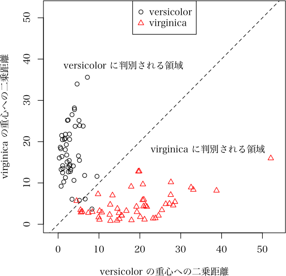
else { # scatterplot 各群の重心までの二乗距離
group <- result$個々の判別$実際の群
group.levels <- levels(group)
distance1 <- result$個々の判別$二乗距離1
distance2 <- result$個々の判別$二乗距離2
max1 <- max(distance1)
max2 <- max(distance2)
max0 <- max(max1, max2)
plot(distance1, distance2, col=col[as.integer(group)], pch=pch[as.integer(group)],
xlim=c(0, max0), xlab=paste(group.levels[1], "の重心への二乗距離"),
ylim=c(0, max0), ylab=paste(group.levels[2], "の重心への二乗距離"), asp=1, ...)
abline(0, 1, lty=2)
text(max1, max2/2, paste(group.levels[2], "に判別される領域"), pos=2)
text(0, max2+strheight("H")*1.5, paste(group.levels[1], "に判別される領域"), pos=4)
legend(x=xpos, y=ypos, legend=group.levels, col=col, pch=pch)
}
}
else {
warning("3群以上の場合にはグラフ表示は用意されていません")
}
}
使用例
> (ans <- sdis(iris[1:4], iris[5]))
出力結果例
有効ケース数: 150
群を表す変数: Species
***** 平均値 *****
setosa versicolor virginica 全体
Sepal.Length 5.006 5.936 6.588 5.843333
Sepal.Width 3.428 2.770 2.974 3.057333
Petal.Length 1.462 4.260 5.552 3.758000
Petal.Width 0.246 1.326 2.026 1.199333
***** プールされた群内相関係数行列 *****
Sepal.Length Sepal.Width Petal.Length Petal.Width
Sepal.Length 1.0000000 0.5302358 0.7561642 0.3645064
Sepal.Width 0.5302358 1.0000000 0.3779162 0.4705346
Petal.Length 0.7561642 0.3779162 1.0000000 0.4844589
Petal.Width 0.3645064 0.4705346 0.4844589 1.0000000
変数編入基準 Pin: 0.05
変数除去基準 Pout: 0.05
編入候補変数: Petal.Length P : <0.001 ***** 編入されました
***** ステップ 1 ***** 編入変数: Petal.Length
***** 分類関数 *****
setosa versicolor virginica 偏F値 P値
Petal.Length -15.789 -46.007 -59.961 1180.2 <0.001
定数項 11.542 97.996 166.451
ウィルクスのΛ: 0.058628
等価なF値: 1180.2
自由度: (2, 147.00)
P値: <0.001
除去候補変数: Petal.Length P : <0.001 ***** 除去されませんでした
編入候補変数: Sepal.Width P : <0.001 ***** 編入されました
***** ステップ 2 ***** 編入変数: Sepal.Width
***** 分類関数 *****
setosa versicolor virginica 偏F値 P値
Petal.Length 2.2578 -36.964 -52.012 1112.954 <0.001
Sepal.Width -60.4980 -30.315 -26.647 43.035 <0.001
定数項 102.0431 120.720 184.008
ウィルクスのΛ: 0.036884
等価なF値: 307.1
自由度: (4, 292.00)
P値: <0.001
除去候補変数: Sepal.Width P : <0.001 ***** 除去されませんでした
編入候補変数: Petal.Width P : <0.001 ***** 編入されました
***** ステップ 3 ***** 編入変数: Petal.Width
***** 分類関数 *****
setosa versicolor virginica 偏F値 P値
Petal.Length -6.1864 -36.4582 -46.174 38.724 <0.001
Sepal.Width -70.5263 -29.7142 -19.714 54.577 <0.001
Petal.Width 49.6370 -2.9737 -34.313 34.569 <0.001
定数項 119.2991 120.7816 192.254
ウィルクスのΛ: 0.024976
等価なF値: 257.5
自由度: (6, 290.00)
P値: <0.001
除去候補変数: Petal.Width P : <0.001 ***** 除去されませんでした
編入候補変数: Sepal.Length P : 0.0103 ***** 編入されました
***** ステップ 4 ***** 編入変数: Sepal.Length
***** 分類関数 *****
setosa versicolor virginica 偏F値 P値
Petal.Length 32.861 -10.423 -25.5331 35.5902 <0.001
Sepal.Width -47.176 -14.145 -7.3706 21.9359 <0.001
Petal.Width 34.797 -12.868 -42.1582 24.9043 <0.001
Sepal.Length -47.088 -31.396 -24.8917 4.7212 0.0103
定数項 170.420 143.508 206.5394
ウィルクスのΛ: 0.023439
等価なF値: 199.15
自由度: (8, 288.00)
P値: <0.001
除去候補変数: Sepal.Length P : 0.0103 ***** 除去されませんでした
===================== 結果 =====================
***** 分類関数 *****
setosa versicolor virginica 偏F値 P値
Petal.Length 32.861 -10.423 -25.5331 35.5902 <0.001
Sepal.Width -47.176 -14.145 -7.3706 21.9359 <0.001
Petal.Width 34.797 -12.868 -42.1582 24.9043 <0.001
Sepal.Length -47.088 -31.396 -24.8917 4.7212 0.0103
定数項 170.420 143.508 206.5394
***** 判別関数 *****
setosa と versicolor の判別
マハラノビスの汎距離: 9.47967
理論的誤判別率: <0.001
判別係数 標準化判別係数
Petal.Length -21.642 -38.0772
Sepal.Width 16.515 7.1745
Petal.Width -23.833 -18.1055
Sepal.Length 7.846 6.4753
定数項 -13.456
setosa と virginica の判別
マハラノビスの汎距離: 13.39346
理論的誤判別率: <0.001
判別係数 標準化判別係数
Petal.Length -29.197 -51.3696
Sepal.Width 19.903 8.6459
Petal.Width -38.478 -29.2311
Sepal.Length 11.098 9.1595
定数項 18.060
versicolor と virginica の判別
マハラノビスの汎距離: 4.14742
理論的誤判別率: 0.0191
判別係数 標準化判別係数
Petal.Length -7.5551 -13.2925
Sepal.Width 3.3872 1.4714
Petal.Width -14.6449 -11.1256
Sepal.Length 3.2524 2.6842
定数項 31.5157
***** 判別結果集計表 ****
判別された群
実際の群 setosa versicolor virginica
setosa 50 0 0
versicolor 0 48 2
virginica 0 1 49
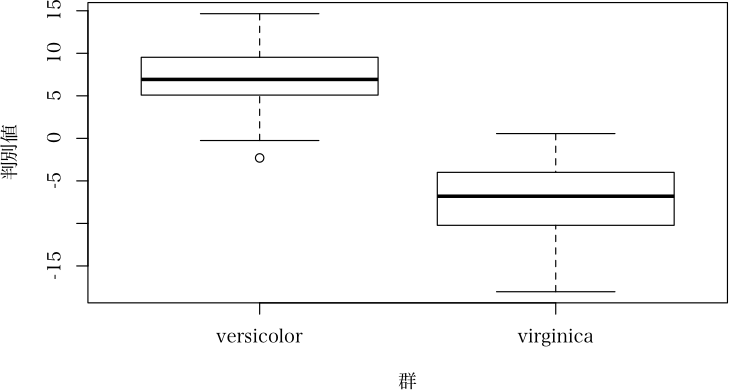
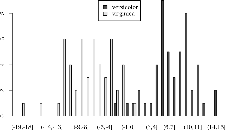
2 群の場合には,plot メソッドでは,以下の3種類の図を描くことができる
> ans2 <- sdis(iris[51:150,1:4], iris[51:150,5], verbose=FALSE)
***** 分類関数 *****
versicolor virginica 偏F値
Petal.Width 1.1729 -23.599 37.0916
Sepal.Width -31.9428 -20.786 10.5875
Petal.Length 5.1633 -8.777 24.1566
Sepal.Length -30.8020 -23.689 7.3679
定数項 123.8859 157.212
P値
Petal.Width < 0.001
Sepal.Width 0.00158
Petal.Length < 0.001
Sepal.Length 0.00789
定数項
***** 判別関数 *****
versicolor と virginica の判別
マハラノビスの汎距離: 3.77079
理論的誤判別率: 0.0297
判別係数 標準化判別係数
Petal.Width -12.3860 -5.2348
Sepal.Width 5.5786 1.8470
Petal.Length -6.9701 -5.7255
Sepal.Length 3.5563 2.3454
定数項 16.6631
***** 判別結果集計表 ****
判別された群
実際の群 versicolor virginica
versicolor 48 2
virginica 1 49
> plot(ans2)
 > plot(ans2, which="barplot", nclass=40, args.legend=list(x="top"))
 > plot(ans2, which="scatterplot", xpos="top")
 解説ページ
解説ページ
直前のページへ戻る E-mail to Shigenobu AOKI
