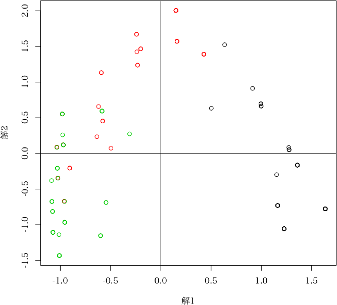
 > plot(ans, which="sample.score", label.cex=0, col=(1:3)[as.integer(iris[,5])]) # サンプルスコアを描画
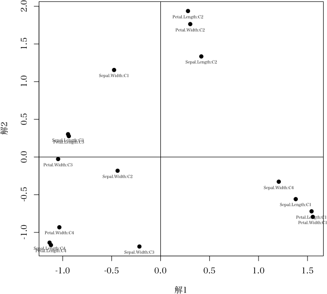
 # corresp 関数を使うときには,qt3 も使う make.dummy 関数により,まえもってカテゴリーデータに変換しておく
インストールは,以下の 1 行をコピーし,R コンソールにペーストする
source("http://aoki2.si.gunma-u.ac.jp/R/src/make.dummy.R", encoding="euc-jp")
# アイテムデータをカテゴリーデータに変換する
make.dummy <- function(dat)
{
ncat <- ncol(dat)
dat[, 1:ncat] <- lapply(dat, function(x) {
if (is.factor(x)) {
return(as.integer(x))
}
else {
return(x)
}
})
mx <- sapply(dat, max)
start <- c(0, cumsum(mx)[1:(ncat-1)])
nobe <- sum(mx)
t(apply(dat, 1, function(obs) 1:nobe %in% (start+obs))) + 0
}
> cat.dat <- make.dummy(dat) # アイテムデータをカテゴリーデータに変換
> cat.dat
Cat-1-1 Cat-1-2 Cat-1-3 Cat-2-1 Cat-2-2 Cat-2-3 Cat-3-1 Cat-3-2 Cat-3-3
[1,] 1 0 0 0 1 0 0 0 1
[2,] 0 0 1 0 1 0 1 0 0
[3,] 0 1 0 0 0 1 1 0 0
[4,] 1 0 0 0 1 0 0 0 1
[5,] 0 1 0 1 0 0 0 1 0
[6,] 0 1 0 0 0 1 0 1 0
> library(MASS)
> corresp(cat.dat, nf=min(nrow(cat.dat), ncol(cat.dat))-1)
# qt3 関数と比較すれば対応はすぐ分かるが,Row/Col scores は列単位に符号が逆転することがある。
# 列単位の符号の逆転は結果の解釈にはなんの影響もない。
# MASS ライブラリの corresp 関数を使ってみた結果
First canonical correlation(s): 9.656767e-01 7.736979e-01 6.015998e-01 3.270135e-01 1.839384e-16
Row scores:
[,1] [,2] [,3] [,4] [,5]
[1,] -1.2038865 -0.7038106 0.2229481 -0.07484681 -1.2217460
[2,] -0.4728660 1.8387224 -1.0573759 0.52673889 -0.9910936
[3,] 0.6932495 0.8004800 1.2836530 -1.49361030 -0.9910936
[4,] -1.2038865 -0.7038106 0.2229481 -0.07484681 -0.7604412
[5,] 1.1425870 -0.9543440 -1.5420864 -0.63693956 -0.9910936
[6,] 1.0448026 -0.2772372 0.8699130 1.75350459 -0.9910936
Column scores:
[,1] [,2] [,3] [,4] [,5]
Cat-1-1 -1.2466766 -0.9096711 0.3705921 -0.2288799 2.4993829
Cat-1-2 0.9943421 -0.1857319 0.3388075 -0.3843320 0.6674281
Cat-1-3 -0.4896733 2.3765380 -1.7576068 1.6107558 1.1216178
Cat-2-1 1.1831983 -1.2334841 -2.5633094 -1.9477470 0.1806949
Cat-2-2 -0.9943421 0.1857319 -0.3388075 0.3843320 -0.2734948
Cat-2-3 0.8999141 0.3381442 1.7898660 0.3973755 0.1806949
Cat-3-1 0.1141083 1.7055769 0.1880628 -1.4783356 0.3605722
Cat-3-2 1.1325683 -0.7959058 -0.5586549 1.7072155 0.3605722
Cat-3-3 -1.2466766 -0.9096711 0.3705921 -0.2288799 -1.0171930
# ca 関数を使ってみる
> ca(cat.dat, nd=min(nrow(cat.dat), ncol(cat.dat))-1)
Principal inertias (eigenvalues):
1 2 3 4 5
Value 0.932531 0.598608 0.361922 0.106938 0
Percentage 46.63% 29.93% 18.1% 5.35% 0%
Rows:
[,1] [,2] [,3] [,4] [,5] [,6]
Mass 0.166667 0.166667 0.166667 0.166667 0.166667 0.166667
ChiDist 1.290994 1.632993 1.290994 1.290994 1.632993 1.290994
Inertia 0.277778 0.444444 0.277778 0.277778 0.444444 0.277778
Dim. 1 -1.203887 -0.472866 0.693249 -1.203887 1.142587 1.044803
Dim. 2 -0.703811 1.838722 0.800480 -0.703811 -0.954344 -0.277237
Dim. 3 0.222948 -1.057376 1.283653 0.222948 -1.542086 0.869913
Dim. 4 -0.074847 0.526739 -1.493610 -0.074847 -0.636940 1.753505
Dim. 5 1.127996 0.997142 0.997142 0.866288 0.997142 0.997142
Columns:
[,1] [,2] [,3] [,4] [,5] [,6]
Mass 0.111111 0.166667 0.055556 0.055556 0.166667 0.111111
ChiDist 1.414214 1.000000 2.236068 2.236068 1.000000 1.414214
Inertia 0.222222 0.166667 0.277778 0.277778 0.166667 0.222222
Dim. 1 -1.246677 0.994342 -0.489673 1.183198 -0.994342 0.899914
Dim. 2 -0.909671 -0.185732 2.376538 -1.233484 0.185732 0.338144
Dim. 3 0.370592 0.338808 -1.757607 -2.563309 -0.338808 1.789866
Dim. 4 -0.228880 -0.384332 1.610756 -1.947747 0.384332 0.397375
Dim. 5 -2.187860 -0.879188 -1.561987 -0.358192 0.324607 -0.358192
[,7] [,8] [,9]
Mass 0.111111 0.111111 0.111111
ChiDist 1.414214 1.414214 1.414214
Inertia 0.222222 0.222222 0.222222
Dim. 1 0.114108 1.132568 -1.246677
Dim. 2 1.705577 -0.795906 -0.909671
Dim. 3 0.188063 -0.558655 0.370592
Dim. 4 -1.478336 1.707216 -0.228880
Dim. 5 0.429670 0.429670 1.055542
# corresp 関数を使うときには,qt3 も使う make.dummy 関数により,まえもってカテゴリーデータに変換しておく
インストールは,以下の 1 行をコピーし,R コンソールにペーストする
source("http://aoki2.si.gunma-u.ac.jp/R/src/make.dummy.R", encoding="euc-jp")
# アイテムデータをカテゴリーデータに変換する
make.dummy <- function(dat)
{
ncat <- ncol(dat)
dat[, 1:ncat] <- lapply(dat, function(x) {
if (is.factor(x)) {
return(as.integer(x))
}
else {
return(x)
}
})
mx <- sapply(dat, max)
start <- c(0, cumsum(mx)[1:(ncat-1)])
nobe <- sum(mx)
t(apply(dat, 1, function(obs) 1:nobe %in% (start+obs))) + 0
}
> cat.dat <- make.dummy(dat) # アイテムデータをカテゴリーデータに変換
> cat.dat
Cat-1-1 Cat-1-2 Cat-1-3 Cat-2-1 Cat-2-2 Cat-2-3 Cat-3-1 Cat-3-2 Cat-3-3
[1,] 1 0 0 0 1 0 0 0 1
[2,] 0 0 1 0 1 0 1 0 0
[3,] 0 1 0 0 0 1 1 0 0
[4,] 1 0 0 0 1 0 0 0 1
[5,] 0 1 0 1 0 0 0 1 0
[6,] 0 1 0 0 0 1 0 1 0
> library(MASS)
> corresp(cat.dat, nf=min(nrow(cat.dat), ncol(cat.dat))-1)
# qt3 関数と比較すれば対応はすぐ分かるが,Row/Col scores は列単位に符号が逆転することがある。
# 列単位の符号の逆転は結果の解釈にはなんの影響もない。
# MASS ライブラリの corresp 関数を使ってみた結果
First canonical correlation(s): 9.656767e-01 7.736979e-01 6.015998e-01 3.270135e-01 1.839384e-16
Row scores:
[,1] [,2] [,3] [,4] [,5]
[1,] -1.2038865 -0.7038106 0.2229481 -0.07484681 -1.2217460
[2,] -0.4728660 1.8387224 -1.0573759 0.52673889 -0.9910936
[3,] 0.6932495 0.8004800 1.2836530 -1.49361030 -0.9910936
[4,] -1.2038865 -0.7038106 0.2229481 -0.07484681 -0.7604412
[5,] 1.1425870 -0.9543440 -1.5420864 -0.63693956 -0.9910936
[6,] 1.0448026 -0.2772372 0.8699130 1.75350459 -0.9910936
Column scores:
[,1] [,2] [,3] [,4] [,5]
Cat-1-1 -1.2466766 -0.9096711 0.3705921 -0.2288799 2.4993829
Cat-1-2 0.9943421 -0.1857319 0.3388075 -0.3843320 0.6674281
Cat-1-3 -0.4896733 2.3765380 -1.7576068 1.6107558 1.1216178
Cat-2-1 1.1831983 -1.2334841 -2.5633094 -1.9477470 0.1806949
Cat-2-2 -0.9943421 0.1857319 -0.3388075 0.3843320 -0.2734948
Cat-2-3 0.8999141 0.3381442 1.7898660 0.3973755 0.1806949
Cat-3-1 0.1141083 1.7055769 0.1880628 -1.4783356 0.3605722
Cat-3-2 1.1325683 -0.7959058 -0.5586549 1.7072155 0.3605722
Cat-3-3 -1.2466766 -0.9096711 0.3705921 -0.2288799 -1.0171930
# ca 関数を使ってみる
> ca(cat.dat, nd=min(nrow(cat.dat), ncol(cat.dat))-1)
Principal inertias (eigenvalues):
1 2 3 4 5
Value 0.932531 0.598608 0.361922 0.106938 0
Percentage 46.63% 29.93% 18.1% 5.35% 0%
Rows:
[,1] [,2] [,3] [,4] [,5] [,6]
Mass 0.166667 0.166667 0.166667 0.166667 0.166667 0.166667
ChiDist 1.290994 1.632993 1.290994 1.290994 1.632993 1.290994
Inertia 0.277778 0.444444 0.277778 0.277778 0.444444 0.277778
Dim. 1 -1.203887 -0.472866 0.693249 -1.203887 1.142587 1.044803
Dim. 2 -0.703811 1.838722 0.800480 -0.703811 -0.954344 -0.277237
Dim. 3 0.222948 -1.057376 1.283653 0.222948 -1.542086 0.869913
Dim. 4 -0.074847 0.526739 -1.493610 -0.074847 -0.636940 1.753505
Dim. 5 1.127996 0.997142 0.997142 0.866288 0.997142 0.997142
Columns:
[,1] [,2] [,3] [,4] [,5] [,6]
Mass 0.111111 0.166667 0.055556 0.055556 0.166667 0.111111
ChiDist 1.414214 1.000000 2.236068 2.236068 1.000000 1.414214
Inertia 0.222222 0.166667 0.277778 0.277778 0.166667 0.222222
Dim. 1 -1.246677 0.994342 -0.489673 1.183198 -0.994342 0.899914
Dim. 2 -0.909671 -0.185732 2.376538 -1.233484 0.185732 0.338144
Dim. 3 0.370592 0.338808 -1.757607 -2.563309 -0.338808 1.789866
Dim. 4 -0.228880 -0.384332 1.610756 -1.947747 0.384332 0.397375
Dim. 5 -2.187860 -0.879188 -1.561987 -0.358192 0.324607 -0.358192
[,7] [,8] [,9]
Mass 0.111111 0.111111 0.111111
ChiDist 1.414214 1.414214 1.414214
Inertia 0.222222 0.222222 0.222222
Dim. 1 0.114108 1.132568 -1.246677
Dim. 2 1.705577 -0.795906 -0.909671
Dim. 3 0.188063 -0.558655 0.370592
Dim. 4 -1.478336 1.707216 -0.228880
Dim. 5 0.429670 0.429670 1.055542
2. カテゴリーデータ行列の場合 > cat.dat <- matrix(c( # 12行10列のカテゴリー行列の例(ファイルから読んでも良い) 0, 0, 1, 0, 0, 0, 0, 0, 0, 0, 0, 0, 1, 1, 1, 0, 0, 0, 0, 0, 1, 1, 1, 1, 1, 1, 1, 1, 1, 1, 1, 1, 1, 0, 0, 0, 1, 0, 0, 0, 1, 1, 1, 1, 0, 0, 1, 1, 1, 0, 1, 1, 1, 1, 1, 1, 1, 0, 1, 0, 1, 1, 1, 1, 0, 1, 1, 1, 1, 1, 1, 1, 1, 1, 0, 1, 1, 0, 0, 0, 1, 0, 0, 0, 0, 1, 0, 0, 0, 0, 1, 1, 1, 0, 0, 0, 0, 0, 0, 0, 1, 1, 0, 0, 0, 1, 1, 0, 0, 0, 1, 0, 0, 0, 0, 1, 0, 0, 0, 0 ), ncol=10, byrow=TRUE) > cat.dat <- data.frame(cat.dat) > cat.dat[,1:10] <- lapply(cat.dat, factor) # factor 変数に変換 > summary(qt3(cat.dat)) $Eigen.value 解1 解2 解3 解4 解5 解6 解7 解8 解9 0.2924314 0.1836443 0.1651647 0.0806121 0.0381495 0.0314432 0.0200612 0.0096876 0.0028926 $Correlation.coefficient 解1 解2 解3 解4 解5 解6 解7 解8 解9 0.540769 0.428537 0.406405 0.283923 0.195319 0.177322 0.141638 0.098426 0.053783 $Category.score 解1 解2 解3 解4 解5 解6 解7 解8 解9 X1 1.12061 0.39097 -0.13398 -0.223139 -0.319548 1.18769 -0.49888 -0.57755 -1.152596 X2 0.25933 0.45437 0.97631 1.046676 0.736518 0.73278 -0.54581 1.13836 1.174476 X3 -0.91129 1.55027 0.45757 -1.304842 -0.056945 -0.44264 0.44628 -0.04614 0.096517 X4 -1.03472 -0.32668 -0.72748 0.555747 -1.182659 -1.03111 -1.79281 0.84489 -0.654223 X5 -1.97313 0.11201 -2.77783 1.052841 1.264068 1.51387 0.69098 -1.11308 0.574480 X6 1.54971 -0.34052 -1.37732 -0.631736 -0.027140 -0.99857 0.48640 0.43337 1.092078 X7 0.22006 -0.10190 0.74101 1.480517 0.392343 -1.40062 0.79666 -1.22887 -0.606862 X8 -0.61293 -2.01552 1.21702 -0.986744 -1.201195 0.58887 -0.87032 -2.22430 2.068638 X9 -0.60676 -1.46512 0.46263 0.042428 -1.327824 0.93432 2.33554 1.54518 -0.735565 X10 -0.53696 -2.43457 0.53113 -2.021192 3.739023 -0.40992 -0.84495 0.70721 -1.598387 $Sample.score 解1 解2 解3 解4 解5 解6 解7 解8 解9 #1 -1.68518 3.617583 1.125886 -4.59577 -0.291551 -2.49626 3.150872 -0.46878 1.79458 #2 -2.41579 1.038881 -2.499758 0.35661 0.041751 0.07541 -1.542789 -1.06453 0.10396 #3 -0.46713 -0.974636 -0.155252 -0.34849 1.032487 0.38047 0.143385 -0.52926 0.48074 #4 0.31839 1.338107 1.255458 0.87983 0.963000 0.10884 0.349920 -1.81405 -2.27055 #5 -0.41362 -0.504573 1.052108 0.30725 -2.164452 0.45864 -0.130456 -0.79600 0.50570 #6 -0.31811 0.079751 -0.731753 0.88866 -0.333548 0.34944 1.693010 1.26512 -0.49201 #7 -0.11362 -1.111969 0.586956 -0.79923 0.428117 -0.52585 -0.382738 0.66847 -0.65267 #8 0.37098 0.632585 -0.026208 0.54194 -0.390328 -1.83515 -1.303990 0.95514 -0.15683 #9 2.46900 0.058866 -1.859360 -1.50547 -0.887492 0.53327 -0.044074 -0.73240 -0.56261 #10 0.28888 1.863404 1.066171 -0.56507 0.614422 2.77804 -1.408320 1.74301 0.73380 #11 1.45613 0.235059 0.126726 1.47251 1.001149 -0.67493 0.420730 -0.59610 2.35715 #12 2.46900 0.058866 -1.859360 -1.50547 -0.887492 0.53327 -0.044074 -0.73240 -0.56261 # MASS ライブラリの corresp 関数を使ってみた結果 > library(MASS) > corresp(cat.dat, nf=min(nrow(cat.dat), ncol(cat.dat))-1) # qt3 関数と比較すれば対応はすぐ分かるが,Row/Col scores は列単位に符号が逆転することがある。 # 列単位の符号の逆転は結果の解釈にはなんの影響もない。 First canonical correlation(s): 0.54076922 0.42853734 0.40640457 0.28392276 0.19531891 0.17732237 0.14163768 0.09842559 0.05378270 Row scores: [,1] [,2] [,3] [,4] [,5] [,6] R 1 -1.6851770 -3.61758251 1.12588635 -4.5957658 0.29155115 -2.4962638 R 2 -2.4157854 -1.03888146 -2.49975810 0.3566057 -0.04175058 0.0754107 R 3 -0.4671300 0.97463551 -0.15525183 -0.3484909 -1.03248691 0.3804732 R 4 0.3183937 -1.33810707 1.25545845 0.8798269 -0.96299989 0.1088441 R 5 -0.4136203 0.50457280 1.05210802 0.3072476 2.16445186 0.4586359 R 6 -0.3181112 -0.07975082 -0.73175256 0.8886619 0.33354815 0.3494440 R 7 -0.1136167 1.11196935 0.58695606 -0.7992338 -0.42811687 -0.5258493 R 8 0.3709833 -0.63258540 -0.02620765 0.5419442 0.39032814 -1.8351460 R 9 2.4690014 -0.05886608 -1.85936019 -1.5054714 0.88749191 0.5332659 R 10 0.2888764 -1.86340447 1.06617112 -0.5650661 -0.61442233 2.7780360 R 11 1.4561265 -0.23505927 0.12672639 1.4725111 -1.00114917 -0.6749329 R 12 2.4690014 -0.05886608 -1.85936019 -1.5054714 0.88749191 0.5332659 [,7] [,8] [,9] R 1 3.15087156 0.4687830 -1.7945774 R 2 -1.54278904 1.0645321 -0.1039616 R 3 0.14338497 0.5292578 -0.4807432 R 4 0.34992015 1.8140517 2.2705462 R 5 -0.13045574 0.7959972 -0.5057021 R 6 1.69300977 -1.2651239 0.4920135 R 7 -0.38273802 -0.6684722 0.6526743 R 8 -1.30399008 -0.9551419 0.1568343 R 9 -0.04407449 0.7324004 0.5626145 R 10 -1.40832024 -1.7430115 -0.7338028 R 11 0.42072965 0.5960950 -2.3571524 R 12 -0.04407449 0.7324004 0.5626145 Col scores: [,1] [,2] [,3] [,4] [,5] [,6] C 1 1.1206082 -0.3909721 -0.1339828 -0.22313884 0.31954755 1.1876881 C 2 0.2593301 -0.4543739 0.9763079 1.04667594 -0.73651791 0.7327791 C 3 -0.9112918 -1.5502692 0.4575654 -1.30484249 0.05694545 -0.4426434 C 4 -1.0347237 0.3266771 -0.7274795 0.55574666 1.18265881 -1.0311084 C 5 -1.9731317 -0.1120064 -2.7778251 1.05284122 -1.26406830 1.5138678 C 6 1.5497117 0.3405195 -1.3773221 -0.63173636 0.02714035 -0.9985682 C 7 0.2200636 0.1018998 0.7410058 1.48051689 -0.39234346 -1.4006218 C 8 -0.6129336 2.0155207 1.2170239 -0.98674384 1.20119463 0.5888707 C 9 -0.6067645 1.4651155 0.4626299 0.04242778 1.32782359 0.9343206 C 10 -0.5369635 2.4345660 0.5311262 -2.02119180 -3.73902292 -0.4099204 [,7] [,8] [,9] C 1 -0.4988845 0.57754601 1.15259565 C 2 -0.5458113 -1.13835704 -1.17447612 C 3 0.4462822 0.04614024 -0.09651722 C 4 -1.7928116 -0.84488665 0.65422318 C 5 0.6909783 1.11307800 -0.57447997 C 6 0.4863993 -0.43337214 -1.09207779 C 7 0.7966612 1.22886718 0.60686215 C 8 -0.8703164 2.22429575 -2.06863847 C 9 2.3355384 -1.54518005 0.73556466 C 10 -0.8449483 -0.70720619 1.59838727 # ca ライブラリの ca 関数を使ってみた結果 > ca(cat.dat, nd=min(nrow(cat.dat), ncol(cat.dat))-1) Principal inertias (eigenvalues): 1 2 3 4 5 6 Value 0.292431 0.183644 0.165165 0.080612 0.038149 0.031443 Percentage 35.49% 22.28% 20.04% 9.78% 4.63% 3.82% 7 8 9 Value 0.020061 0.009688 0.002893 Percentage 2.43% 1.18% 0.35% Rows: [,1] [,2] [,3] [,4] [,5] [,6] Mass 0.016949 0.050847 0.169492 0.067797 0.118644 0.135593 ChiDist 2.357023 1.733832 0.548674 0.875326 0.692660 0.514443 Inertia 0.094162 0.152856 0.051024 0.051945 0.056923 0.035885 Dim. 1 -1.685177 -2.415785 -0.467130 0.318394 -0.413620 -0.318111 Dim. 2 -3.617583 -1.038881 0.974636 -1.338107 0.504573 -0.079751 Dim. 3 1.125886 -2.499758 -0.155252 1.255458 1.052108 -0.731753 Dim. 4 -4.595766 0.356606 -0.348491 0.879827 0.307248 0.888662 Dim. 5 0.291551 -0.041751 -1.032487 -0.963000 2.164452 0.333548 Dim. 6 -2.496264 0.075411 0.380473 0.108844 0.458636 0.349444 Dim. 7 3.150872 -1.542789 0.143385 0.349920 -0.130456 1.693010 Dim. 8 0.468783 1.064532 0.529258 1.814052 0.795997 -1.265124 Dim. 9 -1.794577 -0.103962 -0.480743 2.270546 -0.505702 0.492014 [,7] [,8] [,9] [,10] [,11] [,12] Mass 0.152542 0.101695 0.033898 0.050847 0.067797 0.033898 ChiDist 0.602850 0.540602 1.606905 1.096994 0.939819 1.606905 Inertia 0.055438 0.029720 0.087530 0.061190 0.059882 0.087530 Dim. 1 -0.113617 0.370983 2.469001 0.288876 1.456126 2.469001 Dim. 2 1.111969 -0.632585 -0.058866 -1.863404 -0.235059 -0.058866 Dim. 3 0.586956 -0.026208 -1.859360 1.066171 0.126726 -1.859360 Dim. 4 -0.799234 0.541944 -1.505471 -0.565066 1.472511 -1.505471 Dim. 5 -0.428117 0.390328 0.887492 -0.614422 -1.001149 0.887492 Dim. 6 -0.525849 -1.835146 0.533266 2.778036 -0.674933 0.533266 Dim. 7 -0.382738 -1.303990 -0.044074 -1.408320 0.420730 -0.044074 Dim. 8 -0.668472 -0.955142 0.732400 -1.743011 0.596095 0.732400 Dim. 9 0.652674 0.156834 0.562615 -0.733803 -2.357152 0.562615 Columns: [,1] [,2] [,3] [,4] [,5] [,6] Mass 0.169492 0.135593 0.152542 0.101695 0.050847 0.118644 ChiDist 0.680141 0.602846 0.930789 0.777445 1.631007 1.053797 Inertia 0.078405 0.049278 0.132158 0.061466 0.135264 0.131753 Dim. 1 1.120608 0.259330 -0.911292 -1.034724 -1.973132 1.549712 Dim. 2 -0.390972 -0.454374 -1.550269 0.326677 -0.112006 0.340519 Dim. 3 -0.133983 0.976308 0.457565 -0.727480 -2.777825 -1.377322 Dim. 4 -0.223139 1.046676 -1.304842 0.555747 1.052841 -0.631736 Dim. 5 0.319548 -0.736518 0.056945 1.182659 -1.264068 0.027140 Dim. 6 1.187688 0.732779 -0.442643 -1.031108 1.513868 -0.998568 Dim. 7 -0.498885 -0.545811 0.446282 -1.792812 0.690978 0.486399 Dim. 8 0.577546 -1.138357 0.046140 -0.844887 1.113078 -0.433372 Dim. 9 1.152596 -1.174476 -0.096517 0.654223 -0.574480 -1.092078 [,7] [,8] [,9] [,10] Mass 0.118644 0.050847 0.067797 0.033898 ChiDist 0.615985 1.149112 0.875326 1.453922 Inertia 0.045018 0.067142 0.051945 0.071657 Dim. 1 0.220064 -0.612934 -0.606764 -0.536964 Dim. 2 0.101900 2.015521 1.465116 2.434566 Dim. 3 0.741006 1.217024 0.462630 0.531126 Dim. 4 1.480517 -0.986744 0.042428 -2.021192 Dim. 5 -0.392343 1.201195 1.327824 -3.739023 Dim. 6 -1.400622 0.588871 0.934321 -0.409920 Dim. 7 0.796661 -0.870316 2.335538 -0.844948 Dim. 8 1.228867 2.224296 -1.545180 -0.707206 Dim. 9 0.606862 -2.068638 0.735565 1.598387