目的

度数分布表を与えて，正規分布へのあてはめを行う。指定によっては図を描く。

使用法

fit.normal(f, l, w, accuracy=0, method=c("density", "area"),
           xlab="x", ylab="f(x)", plot=TRUE, col="gray", col1="blue", col2="red")

引数

f            度数を表すベクトル
l            最小の階級の下限値
w            階級幅
accuracy     測定精度（デフォルトは 0）
method       あてはめ方法。確率密度による場合は "density"，面積を計算する場合は "area"
xlab         横軸（測定値）の名称（デフォルトは "x"）
ylab         縦軸の名称（デフォルトは "f(x)"）
plot         図を描くかどうか（デフォルトは TRUE）
col          ヒストグラムの塗りつぶし色（デフォルトは "gray"）
col1         理論正規分布曲線（デフォルトは "blue"）
col2         期待値を描く○の色（デフォルトは "red"）

ソース

インストールは，以下の 1 行をコピーし，R コンソールにペーストする
source("http://aoki2.si.gunma-u.ac.jp/R/src/fit_normal.R", encoding="euc-jp")

# 度数分布表を与えて，正規分布へのあてはめを行い，指定によっては図を描く
fit.normal <- function(      f,                                              # 度数を表すベクトル
                        l,                                              # 最小の階級の下限値
                        w,                                              # 階級幅
                        accuracy=0,                                     # 測定精度
                        method=c("density", "area"),                    # あてはめ方法。確率密度による場合は "density"，面積を計算する場合は "area"
                        xlab="x",                                       # 結果のグラフ表示における横軸の名称
                        ylab="f(x)",                                    # 結果のグラフ表示における縦軸の名称
                        plot=TRUE,                                      # 結果のグラフを描くかどうか
                        col="gray",                                     # ヒストグラムの塗りつぶし色
                        col1="blue",                                    # 理論正規分布曲線の色
                        col2="red")                                     # 期待値を描く○の色
{
        method <- match.arg(method)                                  # 引数の略語を補完する
        f <- c(0, f, 0)                                                      # 度数ベクトルの前後に階級を一つ付加する
        m <- length(f)                                                       # 階級数
        x <- l-accuracy/2-3*w/2+w*(1:m)                                      # 級限界
        names(f) <- as.character(x)                                  # 階級の名称
        n <- sum(f)                                                  # ケース数
        mean <- sum(f*x)/n                                           # 平均値の推定値
        sd <- sqrt(sum(f*x^2)/n-mean^2)                                      # 標準偏差の推定値
        if (method == "area") {                                         # 面積を計算する方法の場合
                z <- (x+w/2-mean)/sd                                 # 級限界の標準得点
                F <- pnorm(z)                                                # 下側確率
                F[m] <- 1                                            # 全部加えたら 1
                p <- F-c(0, F[-m])                                   # 各階級の確率
        }
        else {                                                          # 確率密度による場合
                z <- (x-mean)/sd                                     # 標準得点
                p <- dnorm(z)*w/sd                                   # 確率密度
        }
        exp <- n*p
        if (plot) {                                                     # 結果を図示するときは
                xl <- l+w*-1:(m-1)                                   # 横軸の値
                plot(xl, c(f, 0)/n, type="n", xlab=xlab, ylab=ylab)     # 図の枠組み
                rect(xl, 0, xl+w, c(f, 0)/n, col=col)                   # ヒストグラムの長方形を描く
                points(x, p, col=col2)                                  # 期待値の点を打つ
                x2 <- seq(x[1], x[m], length=100)                    # 理論値
                lines(x2, dnorm(x2, mean, sd)*w, col=col1)              # 理論値の度数多角形を描く
                abline(h=0)                                             # 横軸を描く
        }
        result <- list(method=method, mean=mean, sd=sd, table=cbind(x, f, z, p, exp))
        class(result) <- "fit.normal"                                        # 結果にクラス名を与える
        return(result)
}
print.fit.normal <- function(x)                                              # fit.normal クラスの出力関数
{
        cat("正規分布へのあてはめ (方法 =", x$method, ")\n\n")
        cat(sprintf("推定された　　平均値 = %.7g  標準偏差 = %.7g\n\n", x$mean, x$sd))
        x <- x$table
        cat("   級中心    頻度      z 値       密度      期待値\n")
        for (i in 1:nrow(x)) {
                cat(sprintf("%8.4f %6i %9.3f %9.5f %10.2f\n", x[i,1], as.integer(x[i,2]), x[i,3],  x[i,4], x[i,5]))
        }
        cat(sprintf("     合計 %6i %19.5f %10.2f\n", sum(x[,2]), sum(x[,4]), sum(x[,5])))
}


使用例

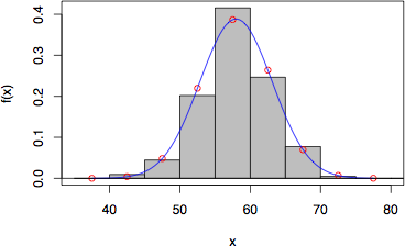
度数分布 f <- c(4, 19, 86, 177, 105, 33, 2) に正規分布をあてはめる

> f <- c(4, 19, 86, 177, 105, 33, 2)

# 面積を計算する方法
# fit.normal は print メソッド（print.fit.normal）を持つ。
> fit.normal(f, 40, 5, method="area")
fit to normal distributution (method = area )

mean = 57.98122  s.d. = 5.133511

x center   freq.      z       p      expectation
 37.5000      0    -3.503   0.00023       0.10
 42.5000      4    -2.529   0.00549       2.34
 47.5000     19    -1.555   0.05428      23.12
 52.5000     86    -0.581   0.22070      94.02
 57.5000    177     0.393   0.37223     158.57
 62.5000    105     1.367   0.26129     111.31
 67.5000     33     2.341   0.07616      32.45
 72.5000      2     3.315   0.00915       3.90
 77.5000      0     4.289   0.00046       0.20
   total    426             1.00000     426.00



# 確率密度を計算する方法
> fit.normal(f, 40, 5, method="density")
fit to normal distributution (method = density )

mean = 57.98122  s.d. = 5.133511

x center   freq.      z       p      expectation
 37.5000      0    -3.990   0.00014       0.06
 42.5000      4    -3.016   0.00412       1.75
 47.5000     19    -2.042   0.04833      20.59
 52.5000     86    -1.068   0.21974      93.61
 57.5000    177    -0.094   0.38686     164.80
 62.5000    105     0.880   0.26376     112.36
 67.5000     33     1.854   0.06964      29.67
 72.5000      2     2.828   0.00712       3.03
 77.5000      0     3.802   0.00028       0.12
   total    426             0.99999     426.00



# fit.normal が返す結果 をprint.fit.normal で書かないときは，
print.default を明示的に使う。

> result <- fit.normal(c(1,2,3,4,5,4,3,2,1),0,1)
> print.default(result)
$method
[1] "density"

$mean
[1] 4.5

$sd
[1] 2

$table
        x f    z          p       exp
-0.5 -0.5 0 -2.5 0.00876415 0.2191038
0.5   0.5 1 -2.0 0.02699548 0.6748871
1.5   1.5 2 -1.5 0.06475880 1.6189699
2.5   2.5 3 -1.0 0.12098536 3.0246341
3.5   3.5 4 -0.5 0.17603266 4.4008166
4.5   4.5 5  0.0 0.19947114 4.9867785
5.5   5.5 4  0.5 0.17603266 4.4008166
6.5   6.5 3  1.0 0.12098536 3.0246341
7.5   7.5 2  1.5 0.06475880 1.6189699
8.5   8.5 1  2.0 0.02699548 0.6748871
9.5   9.5 0  2.5 0.00876415 0.2191038

attr(,"class")
[1] "fit.normal"

 解説ページ