例題：

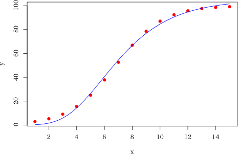
　「表 1 に示すようなデータに曲線をあてはめなさい。」

プログラム：
# quartz(width=500/72, height=350/72)
x <- 1:15
y <- c(2.9, 5.2, 9.1, 15.5, 25, 37.8, 52.6, 66.9,
       78.6, 87, 92.4, 95.7, 97.6, 98.6, 99.2)
dat <- data.frame(x=x, y=y)
# http://aoki2.si.gunma-u.ac.jp/R/simplex.html の，シンプレックス法を使う
model1 <- function(x, p) return(p[1]*p[2]^exp(-p[3]*x))
simplex(model1, c(100, 0.001, 0.1), x, y)
# シンプレックス法で得られた解を初期値として，
# eq. 1: y ~ a*b^exp(-c*x) であてはめる
(ans <- nls(y ~ a*b^exp(-c*x), start=list(a=105, b=0.00016, c=0.37), data=dat))
summary(ans)
plot(x, y, pch=19, col="red")
x2 <- seq(1, 15, by=0.01)
dat2 <- data.frame(x=x2)
y2 <- predict(ans, newdata=dat2)
lines(x2, y2, col="blue")
# eq. 2: y ~ A*exp(-B*C^x) であてはめる（初期値の心配がない）
ans2 <- nls(y ~ SSgompertz(x, A, B, C), data=dat)
p <- ans2$m$getPars()
p[1]       # eq. 1 の a
exp(-p[2]) # eq. 1 の b
-log(p[3]) # eq. 1 の c

実行例：
> x <- 1:15
> y <- c(2.9, 5.2, 9.1, 15.5, 25, 37.8, 52.6, 66.9,
+        78.6, 87, 92.4, 95.7, 97.6, 98.6, 99.2)
> dat <- data.frame(x=x, y=y)
> # http://aoki2.si.gunma-u.ac.jp/R/simplex.html の，シンプレックス法を使う
> model1 <- function(x, p) return(p[1]*p[2]^exp(-p[3]*x))
> simplex(model1, c(100, 0.001, 0.1), x, y)
$converge
[1] TRUE

$parameters
[1] 1.050828e+02 1.571673e-04 3.699247e-01

$residuals
[1] 66.53056

> # シンプレックス法で得られた解を初期値として，
> # eq. 1: y ~ a*b^exp(-c*x) であてはめる
> (ans <- nls(y ~ a*b^exp(-c*x), start=list(a=105, b=0.00016, c=0.37), data=dat))
Nonlinear regression model
  model:  y ~ a * b^exp(-c * x) 
   data:  dat 
        a         b         c 
1.051e+02 1.572e-04 3.699e-01 
 residual sum-of-squares: 66.53

Number of iterations to convergence: 4 
Achieved convergence tolerance: 8.176e-06 
> summary(ans)

Formula: y ~ a * b^exp(-c * x)

Parameters:
   Estimate Std. Error t value Pr(>|t|)    
a 1.051e+02  2.016e+00  52.124 1.63e-15 ***
b 1.572e-04  1.633e-04   0.963    0.355    
c 3.699e-01  2.170e-02  17.050 8.91e-10 ***
---
Signif. codes:  0 ‘***’ 0.001 ‘**’ 0.01 ‘*’ 0.05 ‘.’ 0.1 ‘ ’ 1 

Residual standard error: 2.355 on 12 degrees of freedom

Number of iterations to convergence: 4 
Achieved convergence tolerance: 8.176e-06 

> plot(x, y, pch=19, col="red")
> x2 <- seq(1, 15, by=0.01)
> dat2 <- data.frame(x=x2)
> y2 <- predict(ans, newdata=dat2)
> lines(x2, y2, col="blue")
> # eq. 2: y ~ A*exp(-B*C^x) であてはめる（初期値の心配がない）
> ans2 <- nls(y ~ SSgompertz(x, A, B, C), data=dat)
> p <- ans2$m$getPars()
> p[1]       # y = a*b^exp(-c*x) の a
       A 
105.0826 
> exp(-p[2]) # y = a*b^exp(-c*x) の b
           B 
0.0001571747 
> -log(p[3]) # y = a*b^exp(-c*x) の c
        C 
0.3699248 

演習問題：

応用問題：