目的

シンプレックス法によるパラメータ推定（非線形最小二乗法などに応用する）。

使用法

simplex(fun, start, x, y, MAXIT=10000, EPSILON=1e-7, LO=0.8, HI=1.2, plot.flag=FALSE)

引数

fun       残差平方が最小値となるパラメータを探す目的関数（y = f(x) のような一変数関数）
          使用例を参照のこと
start     パラメータの初期値ベクトル
x         x 値ベクトル
y	  y 値ベクトル
MAXIT     繰り返し数
EPSILON   推定許容誤差
LO，HI    パラメータの初期値ベクトルから 3 組のパラメータベクトルを作るときの倍数
plot.flag TRUE のときには，あてはめ図を描く
...       plot, lines に渡すパラメータ

ソース

インストールは，以下の 1 行をコピーし，R コンソールにペーストする
source("http://aoki2.si.gunma-u.ac.jp/R/src/simplex.R", encoding="euc-jp")

# シンプレックス法によるパラメータ推定
simplex <- function( fun,                                    # 残差平方が最小値となるパラメータを探す目的関数
                        start,                                  # パラメータの初期値ベクトル
                        x,                                      # x 値ベクトル
                        y,                                      # y 値ベクトル
                        MAXIT=10000,                            # 繰り返し数
                        EPSILON=1e-7,                           # 推定許容誤差
                        LO=0.8, HI=1.2,                         # パラメータの初期値ベクトルから 3 組のパラメータベクトルを作るときの倍数
                        plot.flag=FALSE,                        # TRUE のときには，あてはめ図を描く
                        ...)                                    # plot, lines に渡すパラメータ
{
        residual <- function(x, y, p)                                # 残差平方和を求める関数
        {
                return(sum((y-fun(x, p))^2))
        }
        ip3 <- (ip2 <- (ip1 <- (ip <- length(start))+1)+1)+1
        pa <- matrix(start, nrow=ip, ncol=ip3)
        diag(pa) <- diag(pa)*runif(ip, min=LO, max=HI)
        res <- c(sapply(1:ip1, function(i) residual(x, y, pa[, i])), 0, 0)
        for (loops in 1:MAXIT) {
                res0 <- res[1:ip1]
                mx <- which.max(res0)
                mi <- which.min(res0)
                s <- rowSums(pa[, 1:ip1])
                if (res[mx] < EPSILON || res[mi] < EPSILON || (res[mx]-res[mi])/res[mi] < EPSILON) {
                        break
                }
                i <- ip2
                pa[, ip2] <- (2*s-ip2*pa[, mx])/ip
                res[ip2] <- residual(x, y, pa[, ip2])
                if (res[ip2] < res[mi]) {
                        pa[, ip3] <- (3*s-(2*ip1+1)*pa[, mx])/ip
                        res[ip3] <- residual(x, y, pa[, ip3])
                        if (res[ip3] <= res[ip2]) {
                                i <- ip3
                        }
                }
                else if (res[ip2] > res[mx]) {
                        pa[, ip3] <- s/ip1
                        res[ip3] <- residual(x, y, pa[, ip3])
                        if (res[ip3] >= res[mx]) {
                                for (i in which(1:ip1 != mi)) {
                                        pa[, i] <- (pa[, i]+pa[, mi])*0.5
                                        res[i] <- residual(x, y, pa[, i])
                                }
                                i <- 0 # false
                        }
                        else {
                                i <- ip3
                        }
                }
                if (i > 0) {
                        pa[, mx] <- pa[, i]
                        res[mx] <- res[i]
                }
        }
        p <- pa[, mi]
        residuals <- residual(x, y, p)
        if (plot.flag) {
                plot(y ~ x, ...)
                range <- par()$usr
                x <- seq(range[1], range[2], length=1000)
                lines(x, fun(x, p), ...)
        }
        return(list(converge=loops < MAXIT, parameters=p,residuals=residuals))
}


使用例

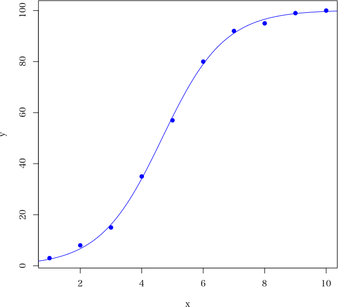
x <- 1:10 # x 値
y <- c(3,8,15,35,57,80,92,95,99,100) # y 値

# あてはめるモデル関数
model1 <- function(x, p)
{
	return(p[1]/(1+p[2]*exp(-p[3]*x)))
}
simplex(model1, c(80, 70, 0.5), x, y, plot.flag=TRUE, col=4, pch=19)

結果は以下の通り（初期値を乱数で決めるので，誤差範囲内で毎回少し違う）

$converge
[1] TRUE

$parameters
[1] 100.1798668 100.9359840   0.9887913

$residuals
[1] 9.999328

以下のような図が描かれる



 解説ページ