散布図(各種の描画機能付き) Last modified: Aug 13, 2009
目的
散布図を描き,棄却楕円(確率楕円),回帰直線,回帰直線の信頼限界帯,MA,RMA による回帰直線を描く。
使用法
scatter(x, y, ellipse=F, lrl=F, cb=F, ma=F, rma=F, alpha=0.05)
引数
x 独立変数(横軸)
y 従属変数(縦軸)
ellipse 確率楕円を描くとき ellipse=TRUE を指定 注
lrl 回帰直線を描くとき lel=TRUE を指定 注
cb 回帰直線の信頼限界帯を描くとき cb=TRUE を指定
ma Major Axis regression による回帰直線を描くとき ma=TRUE を指定 注
rma Reduced Major Axis regression による回帰直線を描くとき rma=TRUE を指定 注
alpha 確率楕円,回帰直線の信頼限界帯を描くときのα。信頼度=(1-α)×100%
acc 確率楕円のなめらかさ
xlab x 軸名称
ylab y 軸名称
注:TRUE/FALSE 以外に,長さ 3 の数値ベクトルで,
(線種, 太さ, 色) を指定できる。数値は lty, lwd, col を参照のこと
棄却楕円のときは,色は,border の色
ソース
インストールは,以下の 1 行をコピーし,R コンソールにペーストする
source("http://aoki2.si.gunma-u.ac.jp/R/src/scatter.R", encoding="euc-jp")
# 散布図を描き,棄却楕円(確率楕円),回帰直線,回帰直線の信頼限界帯,MA,RMA による回帰直線を描く
scatter <- function( x, # 独立変数(横軸にとる)
y, # 従属変数(縦軸にとる)
ellipse=FALSE, # 確率楕円を加えるときに TRUE *1
lrl=FALSE, # 回帰直線を加えるときに TRUE *1
cb=FALSE, # 回帰直線の信頼限界を加えるときに TRUE
ma=FALSE, # MA による回帰直線を加えるときに TRUE *1
rma=FALSE, # RMA による回帰直線を加えるときに TRUE *1
alpha=0.05, # 1-α が信頼度(信頼率)
acc=2000, # 確率楕円のなめらかさ
xlab=NULL, # x 軸名称
ylab=NULL) # y 軸名称
# *1 TRUE/FALSE 以外に,長さ 3 の数値ベクトルで,
# (線種, 太さ, 色) を指定できる。数値は lty, lwd, col を参照のこと
{ # 棄却楕円のときは,色は,border の色
comp <- function(a)
{
if (length(a) == 1) a[2] <- a[3] <- 1
if (length(a) == 2) a[3] <- 1
return(a)
}
ellipse.draw <- function(x, y, alpha, acc, ellipse, # 棄却楕円を描く
xlab, ylab)
{
ellipse <- comp(ellipse)
vx <- var(x)
vy <- var(y)
vxy <- var(x, y)
lambda <- eigen(var(cbind(x, y)))$values
a <- sqrt(vxy^2/((lambda[2]-vx)^2+vxy^2))
b <- (lambda[2]-vx)*a/vxy
theta <- atan(a/b)
k <- sqrt(-2*log(alpha))
l1 <- sqrt(lambda[1])*k
l2 <- sqrt(lambda[2])*k
x2 <- seq(-l1, l1, length.out=acc)
tmp <- 1-x2^2/l1^2
y2 <- l2*sqrt(ifelse(tmp < 0, 0, tmp))
x2 <- c(x2, rev(x2))
y2 <- c(y2, -rev(y2))
s0 <- sin(theta)
c0 <- cos(theta)
xx <- c0*x2+s0*y2+mean(x)
yy <- -s0*x2+c0*y2+mean(y)
rngx <- range(c(x, xx))
rngy <- range(c(y, yy))
plot(rngx, rngy, type="n", xlab=xlab, ylab=ylab)
polygon(xx, yy, lty=ellipse[1], lwd=ellipse[2], border=ellipse[3])
}
conf.limit <- function(x, y, cb, alpha, lrl) # 回帰直線と信頼限界帯を描く
{
lrl <- comp(lrl)
n <- length(x)
b <- var(x, y)/var(x)
a <- mean(y)-b*mean(x)
abline(a, b, lty=lrl[1], lwd=lrl[2], col=lrl[3])
if (cb) {
sx2 <- var(x)*(n-1)
R <- par()$usr # 横軸の範囲
x1 <- seq(R[1], R[2], length.out=2000)
y1 <- a+b*x1
ta <- -qt(alpha/2, n-2)
Ve <- (var(y)-var(x, y)^2/var(x))*(n-1)/(n-2)
temp <- ta*sqrt(Ve)*sqrt(1/n+(x1-mean(x))^2/sx2)
y2 <- y1-temp
lines(x1, y2, lty="dotted")
y2 <- y1+temp
lines(x1, y2, lty="dotted")
temp <- ta*sqrt(Ve)*sqrt(1+1/n+(x1-mean(x))^2/sx2)
y2 <- y1-temp
lines(x1, y2, lty="dashed")
y2 <- y1+temp
lines(x1, y2, lty="dashed")
}
cat("LS(least squares)--------------------\n")
list(intercept=a, slope=b)
}
MA <- function(x, y, ma) # Major Axis regression
{
ma <- comp(ma)
s2 <- cov(cbind(x, y))
b <- s2[1, 2]/(eigen(s2)$values[1]-s2[2, 2])
a <- mean(y)-b*mean(x)
abline(a, b, lty=ma[1], lwd=ma[2], col=ma[3])
cat("MA(major axis)--------------------\n")
list(intercept=a, slope=b)
}
RMA <- function(x, y, rma) # Reduced Major Axis regression
{
rma <- comp(rma)
b <- sign(cor(x, y))*sqrt(var(y)/var(x))
a <- mean(y)-b*mean(x)
abline(a, b, lty=rma[1], lwd=rma[2], col=rma[3])
cat("RMA(reduced major axis)--------------------\n")
list(intercept=a, slope=b)
}
if (is.null(xlab)) xlab <- deparse(substitute(x)) # x 軸名称
if (is.null(ylab)) ylab <- deparse(substitute(y)) # y 軸名称
OK <- complete.cases(x, y) # 欠損値を持つケースを除く
x <- x[OK]
y <- y[OK]
if (ellipse[1]) { # データポイントをマークして棄却楕円を描く
ellipse.draw(x, y, alpha, acc, ellipse, xlab, ylab)
points(x, y)
}
else { # 散布図のみ
plot(x, y, xlab=xlab, ylab=ylab)
}
if (lrl[1]) { # 回帰直線と信頼限界帯
print(conf.limit(x, y, cb, alpha, lrl))
}
if (ma[1]) { # Major Axis regression
print(MA(x, y, ma))
}
if (rma[1]) { # Reduced Major Axis regression
print(RMA(x, y, rma))
}
}
使用例
> x <- c(132, 146, 140, 196, 132, 154, 154, 168, 140, 140, 156, 114, 134, 116, 150, 178, 150, 120, 150, 146)
> y <- c(90, 90, 84, 96, 90, 90, 74, 92, 60, 82, 80, 62, 80, 80, 76, 98, 86, 70, 80, 80)
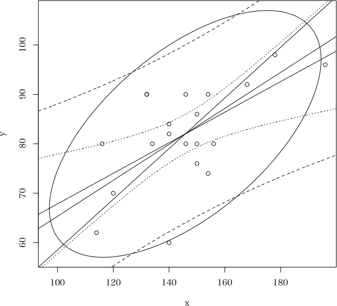
> scatter(x, y, el=TRUE, lrl=TRUE, cb=TRUE, ma=TRUE, rma=TRUE) # 描けるもの全部を描いてみる
LS(least squares)-------------------- # 直線回帰の切片と傾き
$intercept
[1] 36.90722
$slope
[1] 0.3092784
MA(major axis)-------------------- # Major Axis regression による切片と傾き
$intercept
[1] 28.95068
$slope
[1] 0.3638499
RMA(reduced major axis)-------------------- # Reduced Major Axis regression による切片と傾き
$intercept
[1] 7.29765
$slope
[1] 0.5123618
以下のような図が描かれる(傾きの急なものから順に,RMA, MA, 普通の回帰直線)
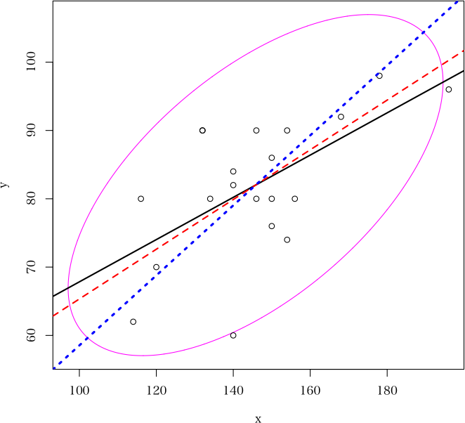
 > scatter(x, y, ellipse=c(1,1,6), lrl=c(1,2,1), ma=c(2,2,2), rma=c(3,3,4)) # 線種,太さ,色の三つ組で指定するとき
 解説ページ
解説ページ
直前のページへ戻る E-mail to Shigenobu AOKI
