Ń–¬–ľ‹ŇŔň°°°°°°°°°°°Last modified: Jun 20, 2008
Ő‹Ň™
ĹÁįŐ•«°ľ•Ņ§ň§ń§§§∆°§Ń–¬–ľ‹ŇŔň°§ň§Ť§Ž≤ÚņŌ§ÚĻ‘§¶
Ľ»Õ—ň°
ro.dual(F)
summary(object, nf=ncol(object), weighted=FALSE, digits=3)
plot(object, first=1, second=2, weighted=FALSE)
įķŅŰ
F ĹÁįŐ•«°ľ•Ņ§ÚĻ‘őů§»§∑§∆ÕŅ§®§Ž
object dual §¨ ÷§Ļ•™•÷•ł•ß•Į•»
nf §§§Į§ń§ő≤Ú§ÚĹ–őŌ§Ļ§Ž§ę° •«•’•©•Ž•»§Ōļ«¬ÁŅŰ°ň
weighted ŃÍīō»ś§«ĹҧŖ…’§Ī§∑§Ņ≤Ú§Ú¬–囧ň§Ļ§Ž§ę§…§¶§ę° •«•’•©•Ž•»§Ō°§ĹҧŖ…’§Ī§∑§ §§≤Ú°ň
digits Ĺ–őŌ§Ļ§ŽŅŰ√Õ§őĺģŅŰŇņį ≤ľ§ő∑ŚŅŰ
first ≤£ľī§ňľŤ§Ž≤Ú§ő»÷Ļś° •«•’•©•Ž•»§Ō 1°ň
second Ĺńľī§ňľŤ§Ž≤Ú§ő»÷Ļś° •«•’•©•Ž•»§Ō 2°ň
color.row Ļ‘§ňÕŅ§®§ť§ž§ŽŅŰ√Õ§Ú…Ń§ĮĶ≠Ļś° •«•’•©•Ž•»§Ō "blue"°ň
color.col őů§ňÕŅ§®§ť§ž§ŽŅŰ√Õ§Ú…Ń§ĮĶ≠Ļś° •«•’•©•Ž•»§Ō "black"°ň
mark.row Ļ‘§ňÕŅ§®§ť§ž§ŽŅŰ√Õ§Ú…Ń§ĮĶ≠Ļś° •«•’•©•Ž•»§Ō 19°ň
mark.col őů§ňÕŅ§®§ť§ž§ŽŅŰ√Õ§Ú…Ń§ĮĶ≠Ļś° •«•’•©•Ž•»§Ō 15°ň
xlab ≤£ļ¬…łľīŐĺ° •«•’•©•Ž•»§Ō paste("Axis", first, sep="-")°ň
ylab Ĺńļ¬…łľīŐĺ° •«•’•©•Ž•»§Ō paste("Axis", second, sep="-")°ň
axis ļ¬…łľī§ÚŇņņĢ§«…ѧĮ§ §ť TRUE° •«•’•©•Ž•»§Ō FALSE°ň
xcgx ≤£ľī§ňľŤ§Žļ¬…ł§ő…šĻś»ŅŇ姨…¨Õ◊§ §ť TRUE° •«•’•©•Ž•»§Ō FALSE°ň
xcgy Ĺńľī§ňľŤ§Žļ¬…ł§ő…šĻś»ŅŇ姨…¨Õ◊§ §ť TRUE° •«•’•©•Ž•»§Ō FALSE°ň
... points, text Ňý§ňŇŌ§Ķ§ž§Ž§Ĺ§ő¬ĺ§őįķŅŰ
•Ĺ°ľ•Ļ
•§•ů•Ļ•»°ľ•Ž§Ō°§į ≤ľ§ő 1 Ļ‘§Ú•≥•‘°ľ§∑°§R •≥•ů•Ĺ°ľ•Ž§ň•ŕ°ľ•Ļ•»§Ļ§Ž
source("http://aoki2.si.gunma-u.ac.jp/R/src/ro.dual.R", encoding="euc-jp")
# ĹÁįŐ•«°ľ•Ņ§ÚŃ–¬–ľ‹ŇŔň°§« ¨ņŌ§Ļ§Ž
ro.dual <- function(F) # ĹÁįŐ•«°ľ•Ņ
{
F <- data.matrix(F) # •«°ľ•Ņ•’•ž°ľ•ŗ§‚Ļ‘őů§ň§Ļ§Ž
N <- nrow(F) # …ĺ≤Ńľ‘§őŅŰ
if (is.null(rownames(F))) { # Ļ‘Őĺ° …ĺ≤Ńľ‘Őĺ°ň§¨§ §§§»§≠°§
row.names <- paste("Row", 1:N, sep="-") # Ļ‘Őĺ§ő šīį
}
n <- ncol(F) # …ĺ≤Ѭ–囧őŅŰ
if (is.null(colnames(F))) { # őůŐĺ° …ĺ≤Ѭ–ĺ›Őĺ°ň§¨§ §§§»§≠°§
col.names <- paste("Col", 1:n, sep="-") # őůŐĺ§ő šīį
}
E <- n+1-2*F
Hn <- t(E)%*%E/(N*n*(n-1)^2)
ans <- eigen(Hn) # ł«Õ≠√Õ°¶ł«Õ≠•Ŕ•Į•»•Ž§ÚĶŠ§Š§Ž
ne <- nrow(Hn)-1 # Õ≠łķ§ ł«Õ≠√Õ°¶ł«Õ≠•Ŕ•Į•»•Ž§őłńŅŰ
eta2 <- ans$values[1:ne] # ł«Õ≠√Õ° ŃÍīō»ś§ő∆ů印ň
eta <- sqrt(eta2) # ŃÍīō»ś
contribution <- eta2/sum(ans$values[1:ne])*100 # īůÕŅő®
cumcont <- cumsum(contribution) # őŖņ—īůÕŅő®
result <- rbind(eta2, eta, contribution, cumcont) # ∑Ž≤Ő
dimnames(result) <- list(c("eta square", "correlation", "contribution", "cumulative contribution"),
paste("Axis", 1:ne, sep="-"))
W <- ans$vectors[, 1:ne, drop=FALSE] # ł«Õ≠•Ŕ•Į•»•Ž
col.score <- W*sqrt(n) # őů•Ļ•≥•Ę
col.score2 <- t(t(col.score)*eta) # ŃÍīō»ś§«ĹҧŖ…’§Ī§∑§Ņőů•Ļ•≥•Ę
row.score2 <- t(t(E%*%W/sqrt(n)/(n-1))) # ŃÍīō»ś§«ĹҧŖ…’§Ī§∑§ŅĻ‘•Ļ•≥•Ę
row.score <- t(t(row.score2)/eta) # Ļ‘•Ļ•≥•Ę
colnames(col.score) <- colnames(row.score) <- colnames(result)
rownames(col.score) <- col.names
rownames(row.score) <- row.names
dimnames(col.score2) <- dimnames(col.score)
dimnames(row.score2) <- dimnames(row.score)
result <- list( result=result,
row.score=row.score,
col.score=col.score,
row.score.weighted=row.score2,
col.score.weighted=col.score2)
class(result) <- "dual" # summary, plot •Š•Ĺ•√•…§¨§Ę§Ž
return(result)
}
•§•ů•Ļ•»°ľ•Ž§Ō°§į ≤ľ§ő 1 Ļ‘§Ú•≥•‘°ľ§∑°§R •≥•ů•Ĺ°ľ•Ž§ň•ŕ°ľ•Ļ•»§Ļ§Ž
source("http://aoki2.si.gunma-u.ac.jp/R/src/summary.dual.R", encoding="euc-jp")
# dual •Į•ť•Ļ §ő§Ņ§Š§ő summary •Š•Ĺ•√•…°°° dual, pc.dual, ro.dual §¨ÕÝÕ—§Ļ§Ž°ň
summary.dual <- function( x, # dual §¨ ÷§Ļ•™•÷•ł•ß•Į•»
nf=ncol(x[[1]]), # Ĺ–őŌ§Ļ§Ž≤Ú§őŅŰ
weighted=FALSE, # ŃÍīō»ś§«ĹҧŖ…’§Ī§∑§Ņ≤Ú§ÚĹ–őŌ§Ļ§Ž§ §ť TRUE
digits=3) # Ĺ–őŌ§Ļ§ŽŅŰ√Õ§őĺģŅŰŇņį ≤ľ§ő∑ŚŅŰ
{
suf <- if (weighted) 4 else 2 # ŃÍīō»ś§«ĹҧŖ…’§Ī§∑§Ņ≤Ú§‚Ń™§Ŕ§Ž
str <- if (weighted) "weighted " else ""
print(round(x[[1]][, 1:nf, drop=FALSE], digits=digits))
cat(sprintf("\n%srow score\n", str))
print(round(x[[suf]][, 1:nf, drop=FALSE], digits=digits))
cat(sprintf("\n%scolumn score\n", str))
print(round(x[[suf+1]][, 1:nf, drop=FALSE], digits=digits))
}
•§•ů•Ļ•»°ľ•Ž§Ō°§į ≤ľ§ő 1 Ļ‘§Ú•≥•‘°ľ§∑°§R •≥•ů•Ĺ°ľ•Ž§ň•ŕ°ľ•Ļ•»§Ļ§Ž
source("http://aoki2.si.gunma-u.ac.jp/R/src/plot.dual.R", encoding="euc-jp")
# dual •Į•ť•Ļ §ő§Ņ§Š§ő plot •Š•Ĺ•√•…°°° dual, pc.dual, ro.dual §¨ÕÝÕ—§Ļ§Ž°ň
plot.dual <- function( x, # dual §¨ ÷§Ļ•™•÷•ł•ß•Į•»
first=1, # ≤£ľī§ň•◊•Ū•√•»§Ļ§Ž≤Ú
second=2, # Ĺńľī§ň•◊•Ū•√•»§Ļ§Ž≤Ú
weighted=FALSE, # ŃÍīō»ś§«ĹҧŖ…’§Ī§∑§Ņ≤Ú§Ú•◊•Ū•√•»§Ļ§Ž§ §ť TRUE
color.row="blue", color.col="black", # Ļ‘§»őů§ő•◊•Ū•√•»Ņß
mark.row=19, mark.col=15, # Ļ‘§»őů§ő•◊•Ū•√•»Ķ≠Ļś
xlab=paste("Axis", first, sep="-"), # ≤£ļ¬…łľīŐĺ
ylab=paste("Axis", second, sep="-"), # Ĺńļ¬…łľīŐĺ
axis=FALSE, # ļ¬…łľī§ÚŇņņĢ§«…ѧĮ§ §ť TRUE
xcgx=FALSE, # ≤£ľī§ňľŤ§Žļ¬…ł§ő…šĻś»ŅŇ姨…¨Õ◊§ §ť TRUE
xcgy=FALSE, # Ĺńľī§ňľŤ§Žļ¬…ł§ő…šĻś»ŅŇ姨…¨Õ◊§ §ť TRUE
...) # points, text Ňý§ňŇŌ§Ķ§ž§Ž§Ĺ§ő¬ĺ§őįķŅŰ
{
if (ncol(x[[1]]) == 1) {
warning("≤Ú§¨1łń§∑§ę§Ę§Í§ř§Ľ§ů°£∆ůľ°łĶ«Ř√÷Ņř§Ō…ѧĪ§ř§Ľ§ů°£")
return
}
suf <- if (weighted) 4 else 2 # ŃÍīō»ś§«ĹҧŖ…’§Ī§∑§Ņ≤Ú§‚Ń™§Ŕ§Ž
old <- par(xpd=TRUE, mar=c(5.1, 5.1, 2.1, 5.1)) # ļłĪ¶§Ú¬Á§≠§Š§ň∂ű§Ī§Ž
row1 <- x[[suf]] [, first] # ≤£ľī§ňľŤ§Ž≤Ú
col1 <- x[[suf+1]][, first]
if (xcgx) { # …¨Õ◊§ §ť…šĻś»ŅŇĺ
row1 <- -row1
col1 <- -col1
}
row2 <- x[[suf]] [, second] # Ĺńľī§ňľŤ§Ž≤Ú
col2 <- x[[suf+1]][, second]
if (xcgy) { # …¨Õ◊§ §ť…šĻś»ŅŇĺ
row2 <- -row2
col2 <- -col2
}
plot(c(row1, col1), c(row2, col2), type="n", xlab=xlab, ylab=ylab, ...)
points(row1, row2, pch=mark.row, col=color.row, ...)
text(row1, row2, labels=names(row1), pos=3, col=color.row, ...)
points(col1, col2, pch=mark.col, col=color.col, ...)
text(col1, col2, labels=names(col1), pos=3, col=color.col, ...)
par(old)
if (axis) { # ļ¬…łľī§ÚŇņņĢ§«…ѧĮ§ §ť§–
abline(v=0, h=0, lty=3, ...)
}
}
Ľ»Õ—ő„
ņĺő§ P.164 §ő•«°ľ•Ņ
F <- matrix(c(
6,1,5,3,2,8,4,7,
3,8,1,6,7,5,4,2,
5,7,1,6,8,2,4,3,
4,6,2,3,8,7,1,5,
2,4,6,3,7,5,1,8,
2,4,5,3,8,7,1,6,
1,7,6,3,8,5,2,4,
7,5,3,1,8,4,6,2,
4,2,7,3,8,6,5,1,
5,1,2,4,7,6,3,8,
6,4,3,2,8,7,5,1,
3,8,4,2,5,6,1,7,
3,2,1,6,4,7,5,8,
5,8,1,4,7,3,6,2), byrow=TRUE, ncol=8)
ans <- ro.dual(F)
summary(ans)
summary(ans, weighted=TRUE)
plot(ans)
Ĺ–őŌ∑Ž≤Őő„
> ans <- ro.dual(F)
> summary(ans) # ŃÍīō»ś§«ĹҧŖ…’§Ī§∑§ §§≤Ú§Ú°§ĺģŅŰŇņį ≤ľ3∑Ś§«Ĺ–őŌ° •«•’•©•Ž•»°ň
Axis-1 Axis-2 Axis-3 Axis-4 Axis-5 Axis-6 Axis-7
eta square 0.141 0.123 0.066 0.055 0.023 0.016 0.005
correlation 0.376 0.350 0.257 0.235 0.150 0.127 0.070
contribution 33.010 28.623 15.361 12.865 5.257 3.738 1.147
cumulative contribution 33.010 61.633 76.993 89.858 95.115 98.853 100.000
row score
Axis-1 Axis-2 Axis-3 Axis-4 Axis-5 Axis-6 Axis-7
Row-1 1.083 -0.995 -1.010 0.672 -1.316 0.738 -0.529
Row-2 -1.401 0.437 0.834 0.646 0.606 1.758 -0.364
Row-3 -1.306 0.686 0.746 0.883 0.837 -1.245 -1.373
Row-4 -1.308 -1.058 0.046 0.637 -0.699 0.484 -1.546
Row-5 -0.344 -1.668 0.322 -0.694 0.495 -1.380 0.483
Row-6 -0.801 -1.606 -0.248 -0.381 0.600 0.251 -0.203
Row-7 -1.224 -0.791 0.370 -1.455 0.524 0.352 1.106
Row-8 -1.089 0.589 -1.448 0.366 -1.226 -1.403 1.237
Row-9 -0.547 -0.076 -2.062 -1.010 1.407 0.552 0.073
Row-10 -0.054 -1.275 -0.598 1.707 0.662 -1.459 -0.303
Row-11 -1.105 0.149 -1.824 0.474 -0.558 0.945 -0.246
Row-12 -0.718 -1.174 1.084 -0.399 -2.094 0.241 0.420
Row-13 0.464 -0.899 0.310 2.060 0.992 1.048 1.967
Row-14 -1.322 1.027 0.345 0.711 -0.482 -0.193 1.443
column score
Axis-1 Axis-2 Axis-3 Axis-4 Axis-5 Axis-6 Axis-7
Col-1 -0.351 -0.839 0.910 -0.764 1.298 0.956 1.470
Col-2 1.256 -0.665 -1.665 0.660 1.241 -0.440 -0.196
Col-3 -0.866 0.248 0.543 2.396 -0.227 0.234 0.212
Col-4 -0.564 -0.598 -1.094 -0.526 -1.763 -0.584 1.184
Col-5 2.004 0.508 0.819 -0.114 -1.094 0.913 -0.106
Col-6 0.041 1.187 0.882 -0.484 0.510 -2.075 0.109
Col-7 -0.588 -1.463 0.634 -0.459 -0.263 -0.158 -1.951
Col-8 -0.932 1.621 -1.028 -0.709 0.298 1.154 -0.723
> summary(ans, weighted=TRUE) # ŃÍīō»ś§«ĹҧŖ…’§Ī§∑§Ņ≤Ú§Ú°§ĺģŅŰŇņį ≤ľ3∑Ś§«Ĺ–őŌ
Axis-1 Axis-2 Axis-3 Axis-4 Axis-5 Axis-6 Axis-7
eta square 0.141 0.123 0.066 0.055 0.023 0.016 0.005
correlation 0.376 0.350 0.257 0.235 0.150 0.127 0.070
contribution 33.010 28.623 15.361 12.865 5.257 3.738 1.147
cumulative contribution 33.010 61.633 76.993 89.858 95.115 98.853 100.000
weighted row score
Axis-1 Axis-2 Axis-3 Axis-4 Axis-5 Axis-6 Axis-7
Row-1 0.407 -0.348 -0.259 0.158 -0.198 0.093 -0.037
Row-2 -0.527 0.153 0.214 0.152 0.091 0.223 -0.026
Row-3 -0.491 0.240 0.191 0.207 0.126 -0.158 -0.096
Row-4 -0.492 -0.371 0.012 0.150 -0.105 0.061 -0.108
Row-5 -0.129 -0.584 0.083 -0.163 0.074 -0.175 0.034
Row-6 -0.301 -0.562 -0.064 -0.089 0.090 0.032 -0.014
Row-7 -0.460 -0.277 0.095 -0.342 0.079 0.045 0.078
Row-8 -0.410 0.206 -0.372 0.086 -0.184 -0.178 0.087
Row-9 -0.206 -0.027 -0.529 -0.237 0.211 0.070 0.005
Row-10 -0.020 -0.447 -0.153 0.401 0.099 -0.185 -0.021
Row-11 -0.416 0.052 -0.468 0.111 -0.084 0.120 -0.017
Row-12 -0.270 -0.411 0.278 -0.094 -0.314 0.030 0.029
Row-13 0.174 -0.315 0.080 0.484 0.149 0.133 0.138
Row-14 -0.497 0.360 0.089 0.167 -0.072 -0.024 0.101
weighted column score
Axis-1 Axis-2 Axis-3 Axis-4 Axis-5 Axis-6 Axis-7
Col-1 -0.132 -0.294 0.233 -0.179 0.195 0.121 0.103
Col-2 0.472 -0.233 -0.427 0.155 0.186 -0.056 -0.014
Col-3 -0.326 0.087 0.139 0.563 -0.034 0.030 0.015
Col-4 -0.212 -0.209 -0.281 -0.124 -0.265 -0.074 0.083
Col-5 0.754 0.178 0.210 -0.027 -0.164 0.115 -0.007
Col-6 0.015 0.416 0.226 -0.114 0.077 -0.263 0.008
Col-7 -0.221 -0.512 0.163 -0.108 -0.039 -0.020 -0.137
Col-8 -0.350 0.568 -0.264 -0.166 0.045 0.146 -0.051
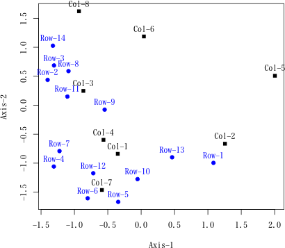
> plot(ans)
 Ľ≤ĻÕ łł•
°°ņĺő§ņŇ…ß°÷ľŃŇ™•«°ľ•Ņ§őŅŰőŐ≤Ĺ°›Ń–¬–ľ‹ŇŔň°§»§Ĺ§őĪĢÕ—°›°◊°§ńęŃ“ĹŮŇĻ°§1982
Ľ≤ĻÕ łł•
°°ņĺő§ņŇ…ß°÷ľŃŇ™•«°ľ•Ņ§őŅŰőŐ≤Ĺ°›Ń–¬–ľ‹ŇŔň°§»§Ĺ§őĪĢÕ—°›°◊°§ńęŃ“ĹŮŇĻ°§1982
 ńĺŃį§ő•ŕ°ľ•ł§ōŐŠ§Ž°°°° E-mail to Shigenobu AOKI
