数量化 II 類 Last modified: Sep 24, 2009
目的
数量化 II 類を行う
使用法
qt2(dat, group)
print.qt2(obj, digits=5)
summary.qt2(obj, digits=5)
plot.qt2(obj, i=1, j=2, xlab=colnames(obj$category.score)[i], ylab=colnames(obj$category.score)[j],
pch=1:obj$ng, col=1:obj$ng, xpos="topright", ypos=NULL,
which=c("boxplot", "barplot", "category.score"), nclass=20, ...)
引数
dat データ行列(行がケース,列が変数)
データは,アイテム変数も factor であること
数値でも良いが,factor にすること
group 最終列が群を表す変数
obj qt2 関数が返すオブジェクト
digits 結果の表示桁数
ソース
インストールは,以下の 1 行をコピーし,R コンソールにペーストする
source("http://aoki2.si.gunma-u.ac.jp/R/src/qt2.R", encoding="euc-jp")
# 数量化 II 類
qt2 <- function(dat, # データ行列(アイテムデータ)
group) # 群変数
{
geneig <- function(a, b) # 一般化固有値問題を解く関数
{
a <- as.matrix(a)
b <- as.matrix(b)
if (nrow(a) == 1) {
res <- list(values=as.vector(a/b), vectors=as.matrix(1))
}
else {
res <- eigen(b)
g <- diag(1/sqrt(res$values))
v <- res$vectors
res <- eigen(g %*% t(v) %*% a %*% v %*% g)
res$vectors <-v %*% g %*% res$vectors
}
return(res)
}
ok <- complete.cases(dat, group)
dat <- subset(dat, ok) # 欠損値を持つケースを除く
group <- group[ok]
stopifnot(all(sapply(dat, is.factor), is.factor(group)))# データは全て factor であること
nc <- nrow(dat) # ケース数
item <- ncol(dat) # アイテム変数の数
n <- as.vector(table(group)) # 各群のケース数
ng <- length(n) # 群の数
vname <- colnames(dat) # 変数名
cname <- unlist(sapply(dat, levels)) # カテゴリー名
gname <- levels(group) # 群の名前
dat <- data.frame(dat, group)
dat[,1:(item+1)] <- lapply(dat, as.integer)
cat <- sapply(dat, max) # 各アイテム変数の最大値
junjo <- c(0, cumsum(cat))[1:(item+1)] # ダミー変数に変換するときに使う,アイテム変数の位置情報
nobe2 <- sum(cat) # 群変数も含めた延べカテゴリー数
nobe <- nobe2-ng # アイテム変数だけの延べカテゴリー数
dat2 <- t(apply(dat, 1, # 群変数も含めて,ダミー変数に変換する
function(obs)
{
zeros <- numeric(nobe2)
zeros[junjo+obs] <- 1
zeros
}
))
a2 <- array(apply(dat2, 1, function(i) outer(i, i)), # クロス集計表を作る準備
dim=c(nobe2, nobe2, nc))
x <- apply(a2, 1:2, sum) # 3 次元配列に対して合計をとる
pcros <- x[1:nobe, 1:nobe] # アイテム変数同士のクロス集計
gcros <- x[(nobe+1):nobe2, 1:nobe] # 群変数とアイテム変数間のクロス集計
w <- outer(n, n)/nc
diag(w) <- 0
grgr <- diag(n-n^2/nc)-w
w <- diag(pcros)
grpat <- gcros-outer(n, w)/nc
pat <- pcros-outer(w, w)/nc
select <- (junjo+1)[1:item] # 冗長な行の添え字
pat <- pat[-select, -select] # 冗長性を排除した行列
grpat <- grpat[-1, -select, drop=FALSE] # 冗長性を排除した行列
r <- grgr[-1, -1, drop=FALSE] # 冗長性を排除した行列
ndim <- ng-1 # 得られる解の数
m <- ncol(pat) # 行列の大きさ
pat <- solve(pat) # 逆行列を求める
c <- grpat%*%pat%*% matrix(t(grpat), nrow=m, ncol=ndim)
w <- geneig(c, r) # 一般化固有値問題を解く
val <- w$values # 固有値
vec <- w$vectors # 固有ベクトル
w <- t(t(pat%*%t(grpat)%*%vec)/sqrt(val))
a <- matrix(0, nrow=nobe, ncol=ndim) # カテゴリースコア
ie <- 0
for (j in 1:item) {
is <- ie+1
ie <- is+cat[j]-2
offset <- junjo[j]+2
a[offset:(offset+ie-is),] <- w[is:ie,]
}
w <- diag(pcros)*a
for (j in 1:item) {
is <- junjo[j]+1
ie <- is+cat[j]-1
s <- colSums(w[is:ie,, drop=FALSE])/nc
a[is:ie,] <- t(t(a[is:ie,])-s)
}
a <- a/sqrt(diag(t(a) %*% pcros %*% a)/nc)
sample.score <- dat2[,1:nobe] %*% a # サンプルスコア
centroid <- n*rbind(0, vec) # 各群の重心
centroid <- t(t(rbind(0, vec))-colSums(centroid)/nc)
centroid <- t(t(centroid)/sqrt(colSums(centroid^2*n)/nc/val))
item1 <- item + 1 # 外的基準との偏相関係数
partial.cor <- matrix(0, item, ndim)
for (l in 1:ndim) {
pat <- matrix(0, item1, item1)
pat[1, 1] <- sum(n*centroid[, l]^2)
temp <- rowSums(a[, l]*t(gcros*centroid[, l]))
pat[1, 2:(item+1)] <- mapply(function(is, ie) sum(temp[is:ie]), junjo[-item1]+1, junjo[-item1]+cat[-item1])
temp <- outer(a[, l], a[, l])*pcros
for (i in 1:item) {
is <- junjo[i]+1
ie <- is+cat[i]-1
for (j in 1:i) {
pat[j+1, i+1] <- sum(temp[is:ie, (junjo[j]+1):(junjo[j]+cat[j])])
}
}
d <- diag(pat)
pat <- pat/sqrt(outer(d, d))
pat <- pat+t(pat)
diag(pat) <- 1
pat <- solve(pat)
partial.cor[, l] <- -pat[2:item1, 1]/sqrt(pat[1, 1]*diag(pat)[-1])
}
dim(val) <- c(1, ndim)
rownames(a) <- paste(rep(vname, cat[1:item]), cname, sep=".")
rownames(partial.cor) <- vname
rownames(centroid) <- gname
rownames(sample.score) <- paste("#", 1:nc, sep="")
rownames(val) <- "Eta"
colnames(val) <- colnames(a) <- colnames(centroid) <- colnames(sample.score) <- colnames(partial.cor) <- paste("解", 1:ndim, sep="")
return(structure(list(ndim=ndim, group=group, ng=ng, category.score=a, partial.cor=partial.cor,
centroid=centroid, eta=val, sample.score=sample.score), class="qt2"))
}
# print メソッド
print.qt2 <- function( obj, # qt2 が返すオブジェクト
digits=5) # 結果の表示桁数
{
cat("\nカテゴリー・スコア\n\n")
print(round(obj$category.score, digits=digits))
}
# summary メソッド
summary.qt2 <- function(obj, # qt2 が返すオブジェクト
digits=5) # 結果の表示桁数
{
print.default(obj, digits=digits)
}
# plot メソッド
plot.qt2 <- function(obj, # qt2 が返すオブジェクト
i=1, # カテゴリースコアを描画するときの対象次元,三群以上の判別図のときの横軸に対する次元
j=2, # 三群以上の判別図のときの縦軸に対する次元
xlab=colnames(obj$category.score)[i], # 三群以上の判別図の横軸のラベル
ylab=colnames(obj$category.score)[j], # 三群以上の判別図の縦軸のラベル
pch=1:obj$ng, # 三群以上の scatterplot を描く記号
col=1:obj$ng, # 三群以上の scatterplot の記号の色
xpos="topright", ypos=NULL, # 三群以上の scatterplot の凡例の位置
which=c("boxplot", "barplot", "category.score"), # 描画するグラフの種類の指定(三群以上の判別のときはこの指示によらない)
nclass=20, # barplot の階級数
...) # plot, boxplot, barplot に引き渡す引数
{
which <- match.arg(which)
if (which == "category.score") {
cscore <- obj$category.score
cname <- rev(rownames(cscore))
cscore <- rev(cscore[, i])
names(cscore) <- NULL
barplot(cscore, horiz=TRUE, xlab=xlab, ...)
text(0, 1.2*(1:length(cname)-0.5), cname, pos=ifelse(cscore > 0, 2, 4))
}
else {
group <- obj$group
if (obj$ndim > 1) {
group.levels <- levels(group)
sample.score <- obj$sample.score
plot(sample.score[, i], sample.score[, j], xlab=xlab, ylab=ylab, col=col[as.integer(group)], pch=pch[as.integer(group)], ...)
legend(x=xpos, y=ypos, legend=group.levels, col=col, pch=pch)
}
else {
if (which == "boxplot") { # boxplot
plot(obj$sample.score[, i] ~ group, xlab="群", ylab="サンプル・スコア", ...)
}
else if (which == "barplot") { # barplot
tbl <- table(group, cut(obj$sample.score,
breaks=pretty(obj$sample.score, n=nclass)))
barplot(tbl, beside=TRUE, legend=TRUE, xlab="サンプル・スコア", ...)
}
}
}
}
使用例
> x1 <- factor(c("hi", "hi", "hi", "med", "med", "hi", "med", "lo"), levels=c("lo", "med", "hi"))
> x2 <- factor(c("female", "male", "female", "male", "male", "male", "male", "female"), levels=c("male", "female"))
> group <- factor(c("Treatment2", "Treatment1", "Treatment1", "Treatment2", "Treatment1", "Control", "Control", "Control"), levels=c("Treatment2", "Treatment1", "Control"))
> dat <- data.frame(x1=x1, x2=x2)
> a <- qt2(dat, group)
> print(a, digits=3) # 実際には print.qt2 関数が使われる
カテゴリー・スコア
解1 解2
x1.lo -3.141 -0.268
x1.med 0.918 -1.195
x1.hi 0.097 0.963
x2.male -0.713 0.656
x2.female 1.188 -1.093
> summary(a) # summary メソッドでは,qt2 が返すすべての結果を返す
$ndim
[1] 2
$group
[1] Treatment2 Treatment1 Treatment1 Treatment2 Treatment1 Control Control Control
Levels: Treatment2 Treatment1 Control
$ng
[1] 3
$category.score
解1 解2
x1.lo -3.14099318 -0.2676973
x1.med 0.91769402 -1.1952703
x1.hi 0.09697778 0.9633770
x2.male -0.71251496 0.6556084
x2.female 1.18752493 -1.0926807
$partial.cor
解1 解2
x1 0.6302492 0.2398440
x2 0.5138933 0.2038242
$centroid
解1 解2
Treatment2 0.7448409 -0.3344828
Treatment1 0.2913815 0.3166733
Control -0.7879421 -0.0936848
$eta
解1 解2
Eta 0.4033555 0.06886674
$sample.score
解1 解2
#1 1.2845027 -0.1293037
#2 -0.6155372 1.6189855
#3 1.2845027 -0.1293037
#4 0.2051791 -0.5396618
#5 0.2051791 -0.5396618
#6 -0.6155372 1.6189855
#7 0.2051791 -0.5396618
#8 -1.9534682 -1.3603781
attr(,"class")
[1] "qt2"
> str(a) # どのような結果が返されるか見てみる
List of 8
$ ndim : num 2
$ group : Factor w/ 3 levels "Treatment2","Treatment1",..: 1 2 2 1 2 3 3 3
$ ng : int 3
$ category.score: num [1:5, 1:2] -3.141 0.918 0.097 -0.713 1.188 ...
..- attr(*, "dimnames")=List of 2
.. ..$ : chr [1:5] "x1:lo" "x1:med" "x1:hi" "x2:male" ...
.. ..$ : chr [1:2] "解1" "解2"
$ partial.cor : num [1:2, 1:2] -0.118 -0.245 0.143 -0.162
..- attr(*, "dimnames")=List of 2
.. ..$ : chr [1:2] "x1" "x2"
.. ..$ : chr [1:2] "解1" "解2"
$ centroid : num [1:3, 1:2] 0.745 0.291 -0.788 -0.334 0.317 ...
..- attr(*, "dimnames")=List of 2
.. ..$ : chr [1:3] "Treatment2" "Treatment1" "Control"
.. ..$ : chr [1:2] "解1" "解2"
$ eta : num [1, 1:2] 0.4034 0.0689
..- attr(*, "dimnames")=List of 2
.. ..$ : chr "Eta"
.. ..$ : chr [1:2] "解1" "解2"
$ sample.score : num [1:8, 1:2] 1.285 -0.616 1.285 0.205 0.205 ...
..- attr(*, "dimnames")=List of 2
.. ..$ : chr [1:8] "#1" "#2" "#3" "#4" ...
.. ..$ : chr [1:2] "解1" "解2"
- attr(*, "class")= chr "qt2"
> print(a$sample.score) # 個々の要素を書き出すこともできる
解1 解2
#1 1.2845027 -0.1293037
#2 -0.6155372 1.6189855
#3 1.2845027 -0.1293037
#4 0.2051791 -0.5396618
#5 0.2051791 -0.5396618
#6 -0.6155372 1.6189855
#7 0.2051791 -0.5396618
#8 -1.9534682 -1.3603781
グラフの表示
> dat <- iris[1:4]
> dat[1:4] <- lapply(iris[1:4], function(x) {qtile <- quantile(x); qtile[1] <- -Inf; qtile[5] <- Inf; cut(x, breaks=qtile, ordered_result=TRUE, labels=paste("C", 1:4, sep=""))})
> group <- iris[,5]
> ans <- qt2(dat, group)
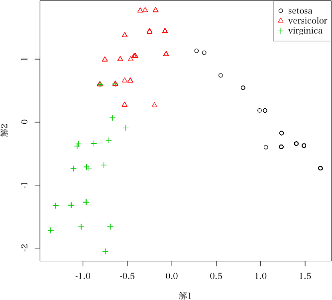
> plot(ans) # 三群以上のときの判別図(ただし,二次元表示のみ)
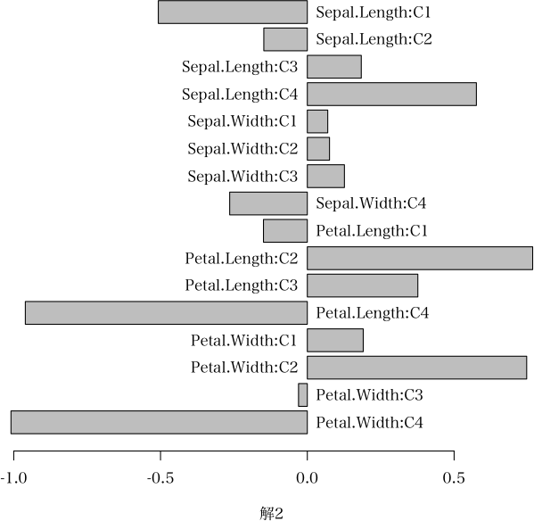
 > plot(ans, which="category.score", i=2) # カテゴリースコアのグラフ化
 > dat <- iris[51:150, 1:4]
> dat[1:4] <- lapply(iris[51:150, 1:4], function(x) {qtile <- quantile(x); qtile[1] <- -Inf; qtile[5] <- Inf; cut(x, breaks=qtile, ordered_result=TRUE, labels=paste("C", 1:4, sep=""))})
> group <- factor(iris[51:150,5], levels=c("versicolor", "virginica"))
> x <- qt2(dat, group)
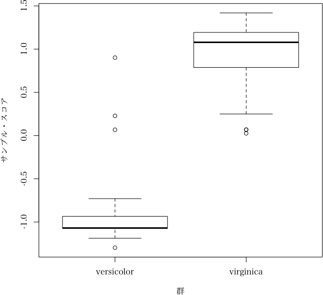
> plot(x)
> dat <- iris[51:150, 1:4]
> dat[1:4] <- lapply(iris[51:150, 1:4], function(x) {qtile <- quantile(x); qtile[1] <- -Inf; qtile[5] <- Inf; cut(x, breaks=qtile, ordered_result=TRUE, labels=paste("C", 1:4, sep=""))})
> group <- factor(iris[51:150,5], levels=c("versicolor", "virginica"))
> x <- qt2(dat, group)
> plot(x)
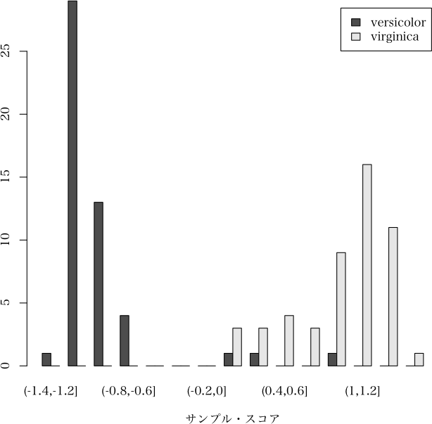
 > plot(x, which="barplot", nclass=10) # 二群判別のときの判別図
 解説ページ
解説ページ
直前のページへ戻る E-mail to Shigenobu AOKI
