双対尺度法 Last modified: Jun 20, 2008
目的
一対比較データについて,双対尺度法による解析を行う
使用法
pc.dual(tbl, one.two=TRUE, col.names=NULL)
summary(object, nf=ncol(object), weighted=FALSE, digits=3)
plot(object, first=1, second=2, weighted=FALSE)
引数
tbl 一対比較データを行列として与える
one.two 一対比較のデータが xi > xj なら 1, xi = xj なら 0,xi < xj なら -1 で入力されていれば FALSE
xi > xj なら 1,xi < xj なら 2, xi = xj なら 0 で入力されていれば TRUE
colnames 評価対象のラベル(デフォルトの NULL なら,便宜的な名前を仮定する)
object dual が返すオブジェクト
nf いくつの解を出力するか(デフォルトは最大数)
weighted 相関比で重み付けした解を対象にするかどうか(デフォルトは,重み付けしない解)
digits 出力する数値の小数点以下の桁数
first 横軸に取る解の番号(デフォルトは 1)
second 縦軸に取る解の番号(デフォルトは 2)
color.row 行に与えられる数値を描く記号(デフォルトは "blue")
color.col 列に与えられる数値を描く記号(デフォルトは "black")
mark.row 行に与えられる数値を描く記号(デフォルトは 19)
mark.col 列に与えられる数値を描く記号(デフォルトは 15)
xlab 横座標軸名(デフォルトは paste("Axis", first, sep="-"))
ylab 縦座標軸名(デフォルトは paste("Axis", second, sep="-"))
axis 座標軸を点線で描くなら TRUE(デフォルトは FALSE)
xcgx 横軸に取る座標の符号反転が必要なら TRUE(デフォルトは FALSE)
xcgy 縦軸に取る座標の符号反転が必要なら TRUE(デフォルトは FALSE)
... points, text 等に渡されるその他の引数
ソース
インストールは,以下の 1 行をコピーし,R コンソールにペーストする
source("http://aoki2.si.gunma-u.ac.jp/R/src/pc.dual.R", encoding="euc-jp")
# 一対比較データを双対尺度法で分析する
pc.dual <- function( F, # 一対比較データ
one.two=TRUE, # 1/2 で入力されているとき 1/-1 に変換する
col.names=NULL) # 評価対象名
{
F <- data.matrix(F) # データフレームも行列にする
if (one.two) { # 1/2 で入力されているとき 1/-1 に変換する
F[F == 2] <- -1
}
N <- nrow(F) # 被調査者数
if (is.null(rownames(F))) { # 被験者の名前が与えられていないとき
row.names <- paste("Row", 1:N, sep="-") # 行ラベルの補完
}
n <- (1+sqrt(1+8*ncol(F)))/2 # 比較対象とされるものの数
if (is.null(col.names)) { # 比較対象の名前が与えられていないとき
col.names <- paste("Col", 1:n, sep="-") # 列ラベルの補完
}
x <- combn(n, 2) # モデル行列作成の添え字
nc <- ncol(x)
A <- matrix(0, nc, n) # モデル行列作成
A[cbind(1:nc, x[1,])] <- 1
A[cbind(1:nc, x[2,])] <- -1
E <- F%*%A
Hn <- t(E)%*%E/(N*n*(n-1)^2)
ans <- eigen(Hn) # 固有値・固有ベクトルを求める
ne <- nrow(Hn)-1 # 有効な固有値・固有ベクトルの個数
eta2 <- ans$values[1:ne] # 固有値(相関比の二乗)
eta <- sqrt(eta2) # 相関比
contribution <- eta2/sum(ans$values[1:ne])*100 # 寄与率
cumcont <- cumsum(contribution) # 累積寄与率
result <- rbind(eta2, eta, contribution, cumcont) # 結果
dimnames(result) <- list(c("eta square", "correlation", "contribution", "cumulative contribution"),
paste("Axis", 1:ne, sep="-"))
W <- ans$vectors[, 1:ne, drop=FALSE] # 固有ベクトル
col.score <- W*sqrt(n) # 列スコア
col.score2 <- t(t(col.score)*eta) # 相関比で重み付けした列スコア
row.score2 <- t(t(E%*%W/sqrt(n)/(n-1))) # 相関比で重み付けした行スコア
row.score <- t(t(row.score2)/eta) # 行スコア
colnames(col.score) <- colnames(row.score) <- colnames(result)
rownames(col.score) <- col.names
rownames(row.score) <- row.names
dimnames(col.score2) <- dimnames(col.score)
dimnames(row.score2) <- dimnames(row.score)
result <- list( result=result,
row.score=row.score,
col.score=col.score,
row.score.weighted=row.score2,
col.score.weighted=col.score2)
class(result) <- "dual" # summary, plot メソッドがある
invisible(result)
}
インストールは,以下の 1 行をコピーし,R コンソールにペーストする
source("http://aoki2.si.gunma-u.ac.jp/R/src/summary.dual.R", encoding="euc-jp")
# dual クラス のための summary メソッド (dual, pc.dual, ro.dual が利用する)
summary.dual <- function( x, # dual が返すオブジェクト
nf=ncol(x[[1]]), # 出力する解の数
weighted=FALSE, # 相関比で重み付けした解を出力するなら TRUE
digits=3) # 出力する数値の小数点以下の桁数
{
suf <- if (weighted) 4 else 2 # 相関比で重み付けした解も選べる
str <- if (weighted) "weighted " else ""
print(round(x[[1]][, 1:nf, drop=FALSE], digits=digits))
cat(sprintf("\n%srow score\n", str))
print(round(x[[suf]][, 1:nf, drop=FALSE], digits=digits))
cat(sprintf("\n%scolumn score\n", str))
print(round(x[[suf+1]][, 1:nf, drop=FALSE], digits=digits))
}
インストールは,以下の 1 行をコピーし,R コンソールにペーストする
source("http://aoki2.si.gunma-u.ac.jp/R/src/plot.dual.R", encoding="euc-jp")
# dual クラス のための plot メソッド (dual, pc.dual, ro.dual が利用する)
plot.dual <- function( x, # dual が返すオブジェクト
first=1, # 横軸にプロットする解
second=2, # 縦軸にプロットする解
weighted=FALSE, # 相関比で重み付けした解をプロットするなら TRUE
color.row="blue", color.col="black", # 行と列のプロット色
mark.row=19, mark.col=15, # 行と列のプロット記号
xlab=paste("Axis", first, sep="-"), # 横座標軸名
ylab=paste("Axis", second, sep="-"), # 縦座標軸名
axis=FALSE, # 座標軸を点線で描くなら TRUE
xcgx=FALSE, # 横軸に取る座標の符号反転が必要なら TRUE
xcgy=FALSE, # 縦軸に取る座標の符号反転が必要なら TRUE
...) # points, text 等に渡されるその他の引数
{
if (ncol(x[[1]]) == 1) {
warning("解が1個しかありません。二次元配置図は描けません。")
return
}
suf <- if (weighted) 4 else 2 # 相関比で重み付けした解も選べる
old <- par(xpd=TRUE, mar=c(5.1, 5.1, 2.1, 5.1)) # 左右を大きめに空ける
row1 <- x[[suf]] [, first] # 横軸に取る解
col1 <- x[[suf+1]][, first]
if (xcgx) { # 必要なら符号反転
row1 <- -row1
col1 <- -col1
}
row2 <- x[[suf]] [, second] # 縦軸に取る解
col2 <- x[[suf+1]][, second]
if (xcgy) { # 必要なら符号反転
row2 <- -row2
col2 <- -col2
}
plot(c(row1, col1), c(row2, col2), type="n", xlab=xlab, ylab=ylab, ...)
points(row1, row2, pch=mark.row, col=color.row, ...)
text(row1, row2, labels=names(row1), pos=3, col=color.row, ...)
points(col1, col2, pch=mark.col, col=color.col, ...)
text(col1, col2, labels=names(col1), pos=3, col=color.col, ...)
par(old)
if (axis) { # 座標軸を点線で描くならば
abline(v=0, h=0, lty=3, ...)
}
}
使用例
西里 P.163 のデータ
F <- matrix(c(
1,1,2,1,1,2,1,2,2,2,2,2,2,2,1,1,2,1,1,1,2,1,1,2,1,2,1,2,
2,2,2,1,2,1,2,1,2,1,2,1,2,2,1,1,1,2,1,1,1,2,2,2,2,1,2,2,
1,1,1,1,1,2,1,1,1,1,1,2,1,1,1,1,2,1,1,1,2,1,2,2,2,2,1,1,
2,1,2,1,1,1,2,1,1,1,1,1,2,2,1,2,2,2,1,1,1,2,2,2,2,2,2,2,
2,2,2,1,2,1,2,2,2,1,2,2,2,2,1,2,1,2,1,1,1,1,2,2,2,1,2,2,
1,1,1,1,1,1,1,2,2,1,2,2,2,2,1,2,2,2,1,1,1,1,2,2,2,2,2,1,
1,1,1,1,1,2,1,1,2,1,1,2,1,2,1,1,2,1,1,1,2,1,2,2,2,2,2,1,
1,1,1,1,1,2,1,1,2,1,2,2,1,2,1,2,2,1,1,2,2,1,2,2,1,2,1,1,
1,2,2,1,1,2,1,2,2,1,1,2,2,1,1,1,2,1,1,1,2,1,2,2,2,2,2,1,
1,2,1,1,2,2,2,2,2,1,2,2,2,1,1,1,1,1,1,2,2,2,2,2,2,1,1,2,
1,2,1,1,1,1,1,2,2,2,2,2,2,1,1,1,1,1,1,1,1,1,2,2,2,2,2,2,
2,2,2,2,1,2,2,1,2,1,1,1,1,2,1,1,1,1,1,1,1,1,1,1,1,2,2,1,
1,2,1,1,2,1,2,2,2,2,2,2,2,1,1,1,1,1,1,2,1,2,2,2,2,1,1,2,
2,2,2,2,1,2,1,2,1,1,1,1,1,1,1,1,1,1,2,1,2,1,1,2,1,2,1,1), byrow=TRUE, nc=28)
ans <- pc.dual(F)
summary(ans)
summary(ans, weighted=TRUE)
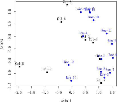
plot(ans)
出力結果例
> ans <- pc.dual(F)
> summary(ans) # 相関比で重み付けしない解を,小数点以下3桁で出力(デフォルト)
Axis-1 Axis-2 Axis-3 Axis-4 Axis-5 Axis-6 Axis-7
eta square 0.141 0.110 0.065 0.055 0.028 0.013 0.006
correlation 0.376 0.331 0.255 0.235 0.169 0.114 0.075
contribution 33.719 26.241 15.591 13.176 6.800 3.122 1.352
cumulative contribution 33.719 59.960 75.550 88.726 95.526 98.648 100.000
row score
Axis-1 Axis-2 Axis-3 Axis-4 Axis-5 Axis-6 Axis-7
Row-1 1.101 -0.417 -0.436 -0.156 1.989 -0.483 -1.119
Row-2 0.334 1.473 1.417 -0.449 -0.520 -0.458 0.510
Row-3 1.211 -1.160 0.105 0.158 -1.527 0.377 0.818
Row-4 0.418 0.507 2.145 0.783 -0.898 1.179 -0.386
Row-5 0.669 1.481 0.872 -0.332 0.255 -1.894 -0.030
Row-6 1.498 0.195 0.345 1.129 0.984 0.226 0.539
Row-7 1.422 -0.968 0.693 0.294 -0.299 0.354 -0.098
Row-8 1.086 -0.927 -0.518 1.193 -0.501 -2.117 1.057
Row-9 1.528 -0.366 0.095 -1.011 -0.122 0.241 -2.161
Row-10 0.808 1.149 -1.173 -0.618 -1.593 -0.316 -1.124
Row-11 1.296 0.613 -0.546 -0.939 1.037 1.691 1.601
Row-12 -0.120 -0.651 1.513 -1.906 0.797 -0.856 0.689
Row-13 0.678 1.453 -1.257 -0.585 -0.387 0.071 0.987
Row-14 -0.024 -1.289 -0.098 -1.995 -0.922 -0.160 0.555
column score
Axis-1 Axis-2 Axis-3 Axis-4 Axis-5 Axis-6 Axis-7
Col-1 1.042 -0.412 -0.488 1.244 0.373 1.364 1.400
Col-2 -0.923 -0.949 1.504 -0.140 -1.563 0.037 0.722
Col-3 0.506 0.361 -1.017 -2.246 -0.468 0.411 0.382
Col-4 0.796 0.248 1.388 -0.443 1.567 -1.240 0.435
Col-5 -1.950 -0.720 -0.721 -0.077 1.403 0.293 -0.317
Col-6 -0.389 1.078 -1.113 0.972 -0.775 -1.644 0.449
Col-7 1.091 -1.380 -0.361 0.326 -0.396 -0.429 -1.824
Col-8 -0.173 1.776 0.807 0.365 -0.140 1.209 -1.246
> summary(ans, weighted=TRUE) # 相関比で重み付けした解を,小数点以下3桁で出力
Axis-1 Axis-2 Axis-3 Axis-4 Axis-5 Axis-6 Axis-7
eta square 0.141 0.110 0.065 0.055 0.028 0.013 0.006
correlation 0.376 0.331 0.255 0.235 0.169 0.114 0.075
contribution 33.719 26.241 15.591 13.176 6.800 3.122 1.352
cumulative contribution 33.719 59.960 75.550 88.726 95.526 98.648 100.000
weighted row score
Axis-1 Axis-2 Axis-3 Axis-4 Axis-5 Axis-6 Axis-7
Row-1 0.414 -0.138 -0.111 -0.037 0.335 -0.055 -0.084
Row-2 0.126 0.488 0.362 -0.105 -0.088 -0.052 0.038
Row-3 0.455 -0.384 0.027 0.037 -0.258 0.043 0.062
Row-4 0.157 0.168 0.548 0.184 -0.151 0.135 -0.029
Row-5 0.251 0.491 0.223 -0.078 0.043 -0.216 -0.002
Row-6 0.563 0.065 0.088 0.265 0.166 0.026 0.041
Row-7 0.534 -0.321 0.177 0.069 -0.050 0.040 -0.007
Row-8 0.408 -0.307 -0.132 0.280 -0.084 -0.242 0.079
Row-9 0.574 -0.121 0.024 -0.237 -0.021 0.028 -0.162
Row-10 0.304 0.381 -0.300 -0.145 -0.269 -0.036 -0.085
Row-11 0.487 0.203 -0.139 -0.220 0.175 0.193 0.120
Row-12 -0.045 -0.216 0.386 -0.448 0.134 -0.098 0.052
Row-13 0.255 0.482 -0.321 -0.137 -0.065 0.008 0.074
Row-14 -0.009 -0.427 -0.025 -0.468 -0.155 -0.018 0.042
weighted column score
Axis-1 Axis-2 Axis-3 Axis-4 Axis-5 Axis-6 Axis-7
Col-1 0.391 -0.137 -0.125 0.292 0.063 0.156 0.105
Col-2 -0.347 -0.315 0.384 -0.033 -0.264 0.004 0.054
Col-3 0.190 0.119 -0.260 -0.527 -0.079 0.047 0.029
Col-4 0.299 0.082 0.355 -0.104 0.264 -0.142 0.033
Col-5 -0.732 -0.239 -0.184 -0.018 0.237 0.033 -0.024
Col-6 -0.146 0.357 -0.284 0.228 -0.131 -0.188 0.034
Col-7 0.410 -0.457 -0.092 0.077 -0.067 -0.049 -0.137
Col-8 -0.065 0.588 0.206 0.086 -0.024 0.138 -0.094
> plot(ans)
 参考文献
西里静彦「質的データの数量化−双対尺度法とその応用−」,朝倉書店,1982
参考文献
西里静彦「質的データの数量化−双対尺度法とその応用−」,朝倉書店,1982
 直前のページへ戻る E-mail to Shigenobu AOKI
