目的

二標本コルモゴロフ・スミルノフ検定を行う

注： R には ks.test という関数が用意されている（原データを用いる）

使用法

ks2(obs1, obs2)
plot.ks2(obj, method=c("barplot", "polygon"), name=c(obj$name1, obj$name2), col=c("grey30", "grey90"),
	 pch=c(19, 2), col2=c(1,4), lty=c(1,2), xlab="", ylab="パーセント", x="topright", y=NULL, ...)				

引数

obs1	第一群の度数分布
obs2	第二群の度数分布

obj                             ks2 関数が返すオブジェクト
method=c("barplot", "polygon")  barplot か度数多角形か
name=c(obj$name1, obj$name2)    凡例に表示する各群の名前
col=c("grey30", "grey90")       barplot の色
pch=c(19, 2)                    度数多角形のマーク
col2=c(1,4)                     度数多角形の線の色
lty=c(1,2)                      度数多角形の線の種類
xlab="", ylab="パーセント"      軸の名称
x="topright", y=NULL            legend の位置
...                             barplot, matplot への引数

ソース

インストールは，以下の 1 行をコピーし，R コンソールにペーストする
source("http://aoki2.si.gunma-u.ac.jp/R/src/ks2.R", encoding="euc-jp")

# 二標本コルモゴロフ・スミルノフ検定を行う
ks2 <- function(     obs1,                                   # 第一群の度数分布
                        obs2)                                   # 第二群の度数分布
{
        stopifnot(length(obs1) == length(obs2))                 # 要素数は同じでなくてはならない
        name1 <- deparse(substitute(obs1))
        name2 <- deparse(substitute(obs2))
        data.name <- paste(name1, "and", name2)
        method <- "二標本コルモゴロフ・スミルノフ検定"
        n1 <- sum(obs1)                                              # 第一群のサンプルサイズ
        n2 <- sum(obs2)                                              # 第二群のサンプルサイズ
        cum1 <- cumsum(obs1)/n1                                      # 第一群の累積相対度数
        cum2 <- cumsum(obs2)/n2                                      # 第二群の累積相対度数
        D <- max(abs(cum1-cum2))                             # 差の絶対値の最大値
        chi <- 4*D^2*n1*n2/(n1+n2)                           # 検定統計量
        df <- 2
        p <- min(1, pchisq(chi, df, lower.tail=FALSE)*2)     # P 値
        stat <- c(D=D, "X-squared"=chi)
        names(df) <- "df"
        return(structure(list(statistic=stat, parameter=df, p.value=p,
                method=method, data.name=data.name,
                obs1=obs1, obs2=obs2, name1=name1, name2=name2),
                class=c("htest", "ks2")))                       # 結果をまとめて返す
}
# plot メソッド（群別の度数分布図を描く）
plot.ks2 <- function(        obj,                                    # ks2 関数が返すオブジェクト
                        method=c("barplot", "polygon"),         # barplot か度数多角形か
                        name=c(obj$name1, obj$name2),           # 各群の名前
                        col=c("grey30", "grey90"),              # barplot の色
                        pch=c(19, 2),                           # 度数多角形のマーク
                        col2=c(1,4),                            # 度数多角形の線の色
                        lty=c(1,2),                             # 度数多角形の線の種類
                        xlab="", ylab="パーセント",             # 軸の名称
                        x="topright", y=NULL,                   # legend の位置
                        ...)                                    # barplot, matplot への引数
{
        d <- rbind(obj$obs1, obj$obs2)
        d <- d/rowSums(d)*100
        nc <- ncol(d)
        if (match.arg(method) == "barplot") {
                barplot(d, beside=TRUE, col=col, ylab=ylab, ...)
                legend(x, y, legend=name, fill=col)
                axis(1, at=1:nc*3-1, labels=1:nc, pos=0)
        }
        else {
                matplot(t(d), type="l", col=col2, lty=lty, xlab=xlab, ylab=ylab, xaxt="n", bty="n", ...)
                points(rep(1:nc, each=2), d, col=rep(col2, nc), pch=rep(pch, nc))
                legend(x, y, legend=name, col=col2, lty=lty, pch=pch)
                axis(1, at=1:nc, labels=1:nc, pos=0)
        }
}


使用例

> obs1 <- c(1, 2, 1, 3, 2, 3, 3, 2, 7, 11, 10, 9, 13, 13, 22, 17, 23, 20, 17, 14, 13, 5, 2, 1, 1, 1)
> obs2 <- c(0, 1, 2, 2, 4, 5, 6, 8, 10, 7, 16, 17, 17, 13, 19, 13, 18, 10, 4, 6, 6, 5, 1, 3, 0, 0)
> (a <- ks2(obs1, obs2))

	二標本コルモゴロフ・スミルノフ検定

data:  obs1 and obs2 
D = 0.1892, X-squared = 14.5969, df = 2, p-value = 0.001353

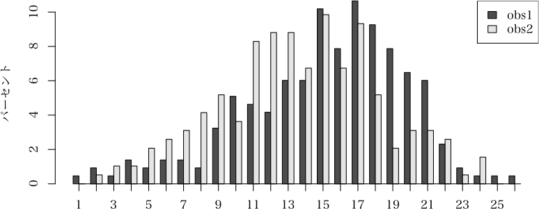
> plot(a)                                    # barplot による度数分布図



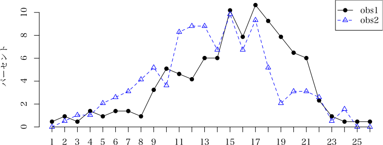
> plot(a, method="polygon")                  # 度数多角形による度数分布図



 解説ページ