双対尺度法 Last modified: Jun 18, 2008
目的
二次元クロス集計表から,双対尺度法による解析を行う
R の MASS ライブラリに入っている corresp 関数と同じであるが,若干親切な出力をする
使用法
dual(tbl)
summary(object, nf=ncol(object), weighted=FALSE, digits=3)
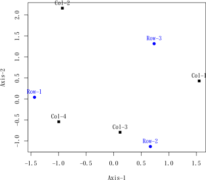
plot(object, first=1, second=2, weighted=FALSE)
引数
tbl 二次元クロス表を行列として与える
object dual が返すオブジェクト
nf いくつの解を出力するか(デフォルトは最大数)
weighted 相関比で重み付けした解を対象にするかどうか(デフォルトは,重み付けしない解)
digits 出力する数値の小数点以下の桁数
first 横軸に取る解の番号(デフォルトは 1)
second 縦軸に取る解の番号(デフォルトは 2)
color.row 行に与えられる数値を描く記号(デフォルトは "blue")
color.col 列に与えられる数値を描く記号(デフォルトは "black")
mark.row 行に与えられる数値を描く記号(デフォルトは 19)
mark.col 列に与えられる数値を描く記号(デフォルトは 15)
xlab 横座標軸名(デフォルトは paste("Axis", first, sep="-"))
ylab 縦座標軸名(デフォルトは paste("Axis", second, sep="-"))
axis 座標軸を点線で描くなら TRUE(デフォルトは FALSE)
xcgx 横軸に取る座標の符号反転が必要なら TRUE(デフォルトは FALSE)
xcgy 縦軸に取る座標の符号反転が必要なら TRUE(デフォルトは FALSE)
... points, text 等に渡されるその他の引数
ソース
インストールは,以下の 1 行をコピーし,R コンソールにペーストする
source("http://aoki2.si.gunma-u.ac.jp/R/src/dual.R", encoding="euc-jp")
# 二次元クロス集計表・度数表を双対尺度法で分析する
dual <- function(tbl) # 二次元クロス表(度数表)を行列として与える
{
tbl <- data.matrix(tbl) # データフレームも行列にする
nr <- nrow(tbl) # 行数
nc <- ncol(tbl) # 列数
if (is.null(rownames(tbl))) { # 行ラベルの補完
rownames(tbl) <- paste("Row", 1:nr, sep="-")
}
if (is.null(colnames(tbl))) { # 列ラベルの補完
colnames(tbl) <- paste("Col", 1:nc, sep="-")
}
ft <- sum(tbl) # サンプルサイズ
fr <- rowSums(tbl) # 行和
fc <- colSums(tbl) # 列和
temp <- sqrt(outer(fc, fc))
w <- t(tbl/fr)%*%tbl/temp-temp/ft
res <- eigen(w) # 固有値・固有ベクトルを求める
ne <- length(res$values[res$values > 1e-5]) # 有効な解の個数
vec <- res$vectors[,1:ne, drop=FALSE] # 固有ベクトルの切り詰め
val <- res$values[1:ne] # 固有値の切り詰め
col.score <- vec*sqrt(ft/fc) # 列スコア
row.score <- tbl%*%col.score/outer(fr, sqrt(val)) # 行スコア
col.score2 <- t(t(col.score)*sqrt(val)) # 相関比で重み付けした列スコア
row.score2 <- t(t(row.score)*sqrt(val)) # 相関比で重み付けした列スコア
cont <- val/sum(diag(w))*100 # 寄与率
chi.sq <- -(ft-1-(nr+nc-1)/2)*log(1-val) # カイ二乗値
df <- nr+nc-1-2*(1:ne) # 自由度
P <- pchisq(chi.sq, df, lower.tail=FALSE) # P 値
result <- matrix(c(val, sqrt(val), cont, cumsum(cont), chi.sq, df, P), byrow=TRUE, ncol=ne)
rownames(result) <- c("eta square", "correlation", "contribution", "cumulative contribution", "Chi square value", "degrees of freedom", "P value")
colnames(result) <- colnames(row.score) <- colnames(col.score) <- paste("Axis", 1:ne, sep="-")
rownames(row.score) <- rownames(tbl)
rownames(col.score) <- colnames(tbl)
dimnames(row.score2) <- dimnames(row.score)
dimnames(col.score2) <- dimnames(col.score)
result <- list(result=result, row.score=row.score, column.score=col.score, row.score.weighted=row.score2, column.score.weighted=col.score2)
class(result) <- c("dual")
invisible(result)
}
インストールは,以下の 1 行をコピーし,R コンソールにペーストする
source("http://aoki2.si.gunma-u.ac.jp/R/src/summary.dual.R", encoding="euc-jp")
# dual クラス のための summary メソッド (dual, pc.dual, ro.dual が利用する)
summary.dual <- function( x, # dual が返すオブジェクト
nf=ncol(x[[1]]), # 出力する解の数
weighted=FALSE, # 相関比で重み付けした解を出力するなら TRUE
digits=3) # 出力する数値の小数点以下の桁数
{
suf <- if (weighted) 4 else 2 # 相関比で重み付けした解も選べる
str <- if (weighted) "weighted " else ""
print(round(x[[1]][, 1:nf, drop=FALSE], digits=digits))
cat(sprintf("\n%srow score\n", str))
print(round(x[[suf]][, 1:nf, drop=FALSE], digits=digits))
cat(sprintf("\n%scolumn score\n", str))
print(round(x[[suf+1]][, 1:nf, drop=FALSE], digits=digits))
}
インストールは,以下の 1 行をコピーし,R コンソールにペーストする
source("http://aoki2.si.gunma-u.ac.jp/R/src/plot.dual.R", encoding="euc-jp")
# dual クラス のための plot メソッド (dual, pc.dual, ro.dual が利用する)
plot.dual <- function( x, # dual が返すオブジェクト
first=1, # 横軸にプロットする解
second=2, # 縦軸にプロットする解
weighted=FALSE, # 相関比で重み付けした解をプロットするなら TRUE
color.row="blue", color.col="black", # 行と列のプロット色
mark.row=19, mark.col=15, # 行と列のプロット記号
xlab=paste("Axis", first, sep="-"), # 横座標軸名
ylab=paste("Axis", second, sep="-"), # 縦座標軸名
axis=FALSE, # 座標軸を点線で描くなら TRUE
xcgx=FALSE, # 横軸に取る座標の符号反転が必要なら TRUE
xcgy=FALSE, # 縦軸に取る座標の符号反転が必要なら TRUE
...) # points, text 等に渡されるその他の引数
{
if (ncol(x[[1]]) == 1) {
warning("解が1個しかありません。二次元配置図は描けません。")
return
}
suf <- if (weighted) 4 else 2 # 相関比で重み付けした解も選べる
old <- par(xpd=TRUE, mar=c(5.1, 5.1, 2.1, 5.1)) # 左右を大きめに空ける
row1 <- x[[suf]] [, first] # 横軸に取る解
col1 <- x[[suf+1]][, first]
if (xcgx) { # 必要なら符号反転
row1 <- -row1
col1 <- -col1
}
row2 <- x[[suf]] [, second] # 縦軸に取る解
col2 <- x[[suf+1]][, second]
if (xcgy) { # 必要なら符号反転
row2 <- -row2
col2 <- -col2
}
plot(c(row1, col1), c(row2, col2), type="n", xlab=xlab, ylab=ylab, ...)
points(row1, row2, pch=mark.row, col=color.row, ...)
text(row1, row2, labels=names(row1), pos=3, col=color.row, ...)
points(col1, col2, pch=mark.col, col=color.col, ...)
text(col1, col2, labels=names(col1), pos=3, col=color.col, ...)
par(old)
if (axis) { # 座標軸を点線で描くならば
abline(v=0, h=0, lty=3, ...)
}
}
使用例
tbl <- matrix(c( # 3行4列の分割表の例(ファイルから読んでも良い)
2, 3, 5, 6,
5, 1, 7, 5,
5, 3, 4, 3
), byrow=TRUE, ncol=4)
ans <- dual(tbl)
summary(ans)
summary(ans, weighted=TRUE)
plot(ans, 1, 2)
library(MASS) # R の MASS 中の corresp を使ってみる
corresp(tbl, nf=min(nrow(tbl), ncol(tbl))-1)
出力結果例
> ans <- dual(tbl)
> summary(ans) # 相関比で重み付けしない解を,小数点以下3桁で出力(デフォルト)
Axis-1 Axis-2
eta square 0.049 0.038
correlation 0.221 0.194
contribution 56.572 43.428
cumulative contribution 56.572 100.000
Chi square value 2.263 1.727
degrees of freedom 4.000 2.000
P value 0.687 0.422
row score
Axis-1 Axis-2
Row-1 -1.436 0.040
Row-2 0.665 -1.131
Row-3 0.733 1.315
column score
Axis-1 Axis-2
Col-1 1.550 0.429
Col-2 -0.930 2.160
Col-3 0.116 -0.792
Col-4 -0.996 -0.542
> summary(ans, weighted=TRUE) # 相関比で重み付けした解
Axis-1 Axis-2
eta square 0.049 0.038
correlation 0.221 0.194
contribution 56.572 43.428
cumulative contribution 56.572 100.000
Chi square value 2.263 1.727
degrees of freedom 4.000 2.000
P value 0.687 0.422
weighted row score
Axis-1 Axis-2
Row-1 -0.318 0.008
Row-2 0.147 -0.220
Row-3 0.162 0.255
weighted column score
Axis-1 Axis-2
Col-1 0.343 0.083
Col-2 -0.206 0.419
Col-3 0.026 -0.154
Col-4 -0.221 -0.105
> plot(ans, 1, 2) # 結果の表示
 > ans # print メソッドでは dual が返す全ての結果を表示する
$result
Axis-1 Axis-2
eta square 0.04905396 0.03765652
correlation 0.22148129 0.19405288
contribution 56.57212279 43.42787721
cumulative contribution 56.57212279 100.00000000
Chi square value 2.26340816 1.72727308
degrees of freedom 4.00000000 2.00000000
P value 0.68743886 0.42162603
$row.score
Axis-1 Axis-2
Row-1 -1.4355847 0.03995533
Row-2 0.6650934 -1.13131472
Row-3 0.7331783 1.31495864
$column.score
Axis-1 Axis-2
Col-1 1.5502397 0.4286333
Col-2 -0.9301824 2.1595197
Col-3 0.1158234 -0.7921783
Col-4 -0.9960553 -0.5418132
$row.score.weighted
Axis-1 Axis-2
Row-1 -0.3179552 0.007753447
Row-2 0.1473057 -0.219534884
Row-3 0.1623853 0.255171517
$column.score.weighted
Axis-1 Axis-2
Col-1 0.34334909 0.08317752
Col-2 -0.20601799 0.41906103
Col-3 0.02565271 -0.15372449
Col-4 -0.22060761 -0.10514041
attr(,"class")
[1] "dual"
> ans # print メソッドでは dual が返す全ての結果を表示する
$result
Axis-1 Axis-2
eta square 0.04905396 0.03765652
correlation 0.22148129 0.19405288
contribution 56.57212279 43.42787721
cumulative contribution 56.57212279 100.00000000
Chi square value 2.26340816 1.72727308
degrees of freedom 4.00000000 2.00000000
P value 0.68743886 0.42162603
$row.score
Axis-1 Axis-2
Row-1 -1.4355847 0.03995533
Row-2 0.6650934 -1.13131472
Row-3 0.7331783 1.31495864
$column.score
Axis-1 Axis-2
Col-1 1.5502397 0.4286333
Col-2 -0.9301824 2.1595197
Col-3 0.1158234 -0.7921783
Col-4 -0.9960553 -0.5418132
$row.score.weighted
Axis-1 Axis-2
Row-1 -0.3179552 0.007753447
Row-2 0.1473057 -0.219534884
Row-3 0.1623853 0.255171517
$column.score.weighted
Axis-1 Axis-2
Col-1 0.34334909 0.08317752
Col-2 -0.20601799 0.41906103
Col-3 0.02565271 -0.15372449
Col-4 -0.22060761 -0.10514041
attr(,"class")
[1] "dual"
> library(MASS)
> corresp(tbl, nf=min(nrow(tbl), ncol(tbl))-1)
# dual 関数と比較すれば対応はすぐ分かるが,Row/Col scores は列単位に符号が逆転することがある。
# 列単位の符号の逆転は結果の解釈にはなんの影響もない。
First canonical correlation(s): 0.2214813 0.1940529 # dual 関数の出力の correl
Row scores: # dual 関数の出力の $"row.score"
[,1] [,2]
R 1 1.4355847 -0.03995533
R 2 -0.6650934 1.13131472
R 3 -0.7331783 -1.31495864
Col scores: # dual 関数の出力の $"column.score"
[,1] [,2]
C 1 -1.5502397 -0.4286333
C 2 0.9301824 -2.1595197
C 3 -0.1158234 0.7921783
C 4 0.9960553 0.5418132
参考文献
西里静彦「質的データの数量化−双対尺度法とその応用−」,朝倉書店,1982
 直前のページへ戻る E-mail to Shigenobu AOKI
