目的

Reduced Major Axis regression を計算する。

使用法

RMA(x, y)

# print メソッド
print.RMA(obj, digits=5, sig=0.95)

# plot メソッド
plot.RMA(obj, posx="topleft", posy=NULL, xlab=obj$names.xy[1], ylab=obj$names.xy[2],	...)

引数

x，y	      2 変数。
	      RMA では，通常の回帰式と違い x，y は完全に対称的（式を変形するだけで y= にも x= にもなる）。
obj           "RMA" オブジェクト
digits        表示桁数
sig           信頼度（デフォルトで 95% 信頼限界）
posx, posy    legend 関数のための位置引数（"topleft", "bottomright" なども可）
xlab, ylab    軸の名前
...           plot 関数に渡されるその他の引数

ソース

インストールは，以下の 1 行をコピーし，R コンソールにペーストする
source("http://aoki2.si.gunma-u.ac.jp/R/src/RMA.R", encoding="euc-jp")

# Reduced Major Axis regression
RMA <- function(x, y)                                                        # 2 つの変数
{
        names.xy <- c(deparse(substitute(x)), deparse(substitute(y)))        # 変数名を控えておく
        OK <- complete.cases(x, y)                                   # 欠損値を持つケースを除く
        x <- x[OK]
        y <- y[OK]
        n <- length(x)                                                       # ケース数
        n1 <- n-1
        df <- n-2                                                    # 信頼限界を求めるときに必要な t 分布の自由度
        slope <- sign(cor(x, y))*sd(y)/sd(x)                         # 傾き
        intercept <- mean(y)-slope*mean(x)                           # 切片
        MSE <- (var(y)-cov(x, y)^2/var(x))*n1/df                     # 標準誤差
        SE.intercept <- sqrt(MSE*(1/n+mean(x)^2/var(x)/n1))          # 切片の標準誤差
        SE.slope <- sqrt(MSE/var(x)/n1)                                      # 傾きの標準誤差
        result <- list(names.xy=names.xy, x=x, y=y,
                       intercept=intercept, SE.intercept=SE.intercept,
                       slope=slope, SE.slope=SE.slope)
        class(result) <- "RMA"
        return(result)
}
# print メソッド
print.RMA <- function(       obj,                                            # "RMA" オブジェクト
                        digits=5,                                       # 表示桁数
                        sig=0.95)                                       # 信頼度
{
        alpha <- (1-sig)/2
        df <- length(obj$x)-2
        intercept <- obj$intercep
        slope <- obj$slope
        SE.intercept <- obj$SE.intercept
        SE.slope <- obj$SE.slope
        CLintercept <- intercept+qt(c(alpha, 1-alpha), df)*SE.intercept      # 切片の信頼限界値
        CLslope <- slope+qt(c(alpha, 1-alpha), df)*SE.slope          # 傾きの信頼限界値
        ans <- data.frame(c(intercept, slope), c(SE.intercept, SE.slope),
                          c(CLintercept[1], CLslope[1]), c(CLintercept[2], CLslope[2]))
        dimnames(ans) <- list(c("Intercept:", "Slope:"),
                              c("Estimate", "S.E.", paste(c(alpha, 1-alpha), "%", sep="")))
        print(ans, digits=digits)               
}
# plot メソッド
plot.RMA <- function(        obj,                                            # "RMA" オブジェクト
                        posx="topleft", posy=NULL,                      # legend 関数のための位置引数
                        xlab=obj$names.xy[1],                           # x 軸の名前
                        ylab=obj$names.xy[2],                           # y 軸の名前
                        ...)                                            # その他の任意の plot 関数の引数

{
        plot(obj$x, obj$y, xlab=xlab, ylab=ylab, ...)
        abline(obj$intercept, obj$slope)
        abline(lm(obj$y~obj$x), lty=2, col=2)
        legend(posx, posy, legend=c("Reduced Major Axis", "linear regression"), lty=1:2, col=1:2)
}


使用例

> y <- c(61, 37, 65, 69, 54, 93, 87, 89, 100, 90, 97)
> x <- c(14, 17, 24, 25, 27, 33, 34, 37, 40, 41, 42)

> (a <- RMA(x, y)) # 出力には print.RMA が使われる

           Estimate     S.E.   0.025%  0.975%
Intercept:  12.1938 10.54975 -11.6714 36.0590
Slope:       2.1194  0.33250   1.3672  2.8715

> print(a, sig=0.9) # 信頼率を指定できる（90% 信頼限界は 0.9 と指定）

           Estimate     S.E.   0.05%   0.95%
Intercept:  12.1938 10.54975 -7.1451 31.5327
Slope:       2.1194  0.33250  1.5099  2.7289

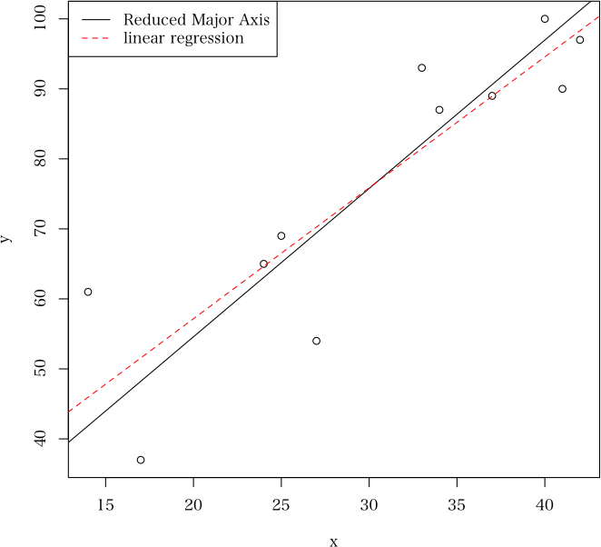
> plot(a) # 散布図の描画には，plot.RMA が使われる