目的

Major Axis regression（主成分回帰）を行う

使用法

MA(x, y)

# print メソッド
print.MA(obj, digits=5, sig=0.95)

# plot メソッド
plot.MA(obj, posx="topleft", posy=NULL, xlab=obj$names.xy[1], ylab=obj$names.xy[2],	...)

引数

x，y	      2 変数。
              通常の回帰式と違い x，y は完全に対称的（式を変形するだけで y= にも x= にもなる）。
obj           "MA" オブジェクト
digits        表示桁数
sig           信頼度（デフォルトで 95% 信頼限界）
posx, posy    legend 関数のための位置引数（"topleft", "bottomright" なども可）
xlab, ylab    軸の名前
...           plot 関数に渡されるその他の引数

ソース

インストールは，以下の 1 行をコピーし，R コンソールにペーストする
source("http://aoki2.si.gunma-u.ac.jp/R/src/MA.R", encoding="euc-jp")

# Major Axis regression（主成分回帰）
MA <- function(x, y)                                                 # 2 つの変数
{
        names.xy <- c(deparse(substitute(x)), deparse(substitute(y)))        # 変数名を控えておく
        OK <- complete.cases(x, y)                                   # 欠損値を持つケースを除く
        x <- x[OK]
        y <- y[OK]
        s2 <- cov(cbind(x, y))                                               # 分散・共分散行列
        ev <- eigen(s2)$values                                               # 固有値
        b <- s2[1, 2]/(ev[1]-s2[2, 2])                                       # 傾き
        a <- mean(y)-b*mean(x)                                               # 切片
        result <- list(names.xy=names.xy, x=x, y=y, ev=ev, intercept=a, slope=b)
        class(result) <- "MA"
        return(result)
}
# print メソッド
print.MA <- function(        obj,                                            # "MA" オブジェクト
                        digits=5,                                       # 表示桁数
                        sig=0.95)                                       # 信頼度
{
        n <- length(obj$x)                                           # ケース数
        ev <- obj$ev
        H <- qf(sig, 1, n-2)/(ev[1]/ev[2]+ev[2]/ev[1]-2)/(n-2)
        CL <- tan(atan(obj$slope)+c(-0.5, 0.5)*asin(2*sqrt(H)))                      # 傾きの信頼限界値
        ans <- data.frame(c(obj$intercept, obj$slope),
                          c(NA, CL[1]), c(NA, CL[2]))
        alpha <- 0.5-sig/2
        dimnames(ans) <- list(c("Intercept:", "Slope:"),
                              c("Estimate", paste(c(alpha, 1-alpha), "%", sep="")))
        print(ans, digits=digits)               
}
# plot メソッド
plot.MA <- function( obj,                                            # "MA" オブジェクト
                        posx="topleft", posy=NULL,                      # legend 関数のための位置引数
                        xlab=obj$names.xy[1],                           # x 軸の名前
                        ylab=obj$names.xy[2],                           # y 軸の名前
                        ...)                                            # その他の任意の plot 関数の引数

{
        plot(obj$x, obj$y, xlab=xlab, ylab=ylab, ...)
        abline(obj$intercept, obj$slope)
        abline(lm(obj$y~obj$x), lty=2, col=2)
        legend(posx, posy, legend=c("Major Axis", "linear regression"), lty=1:2, col=1:2)
}


使用例

> x <- c(14.40, 15.20, 11.30, 2.50, 22.70, 14.90, 1.41, 15.81, 4.19, 15.39, 17.25, 9.52)
> y <- c(159, 179, 100, 45, 384, 230, 100, 320, 80, 220, 320, 210)

> MA(x, y) # 結果の出力には print.MA が使われる

           Estimate 0.025% 0.975%
Intercept:  -32.552     NA     NA
Slope:       18.936 13.439 31.993

> x <- MA(x, y) # 結果を変数に付値する

> print(x, sig=0.99) # print メソッドで，信頼度を指定することができる

           Estimate 0.005% 0.995%
Intercept:  -32.552     NA     NA
Slope:       18.936 11.967 45.138

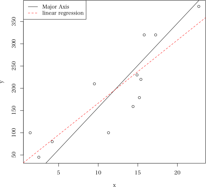
> plot(x) # 散布図と MA による回帰直線を描く